DEMOINTLAB_SPARSE General sparse linear and nonlinear systems in INTLAB

With Version 14 of INTLAB we introduce verification methods for sparse systems of linear and nonlinear equations as well as underdetermined systems and least squares problems.

Sparse linear systems
Verification is sometimes faster than approximation
Methods for sparse matrices
A complex linear system and comparison verifylssSparse1 and 2
A linear system with interval data
A problem where verifylssSparse1 fails but verifylssSparse2 is successful
Equilibration may be counterproductive
A least squares problem
Underdetermined linear systems
Systems of nonlinear equations
Local minumum of a function f:R^n->R
Enjoy INTLAB

Sparse linear systems

There are two algorithms for sparse linear systems, namely verifylssSparse1 based on

S.M. Rump: Verified error bounds for sparse systems Part I: The splitting of a matrix into two factors, to appear

and verifylssSparse2 based on

S.M. Rump: Verified error bounds for sparse systems Part II: Inertia-based bounds, least squares and nonlinear systems, to appear

Problem = 
  struct with fields:

      name: 'VDOL/freeFlyingRobot_5'
     title: 'freeFlyingRobot optimal control problem (matrix 5 of 16)'
         A: [2878×2878 double]
         b: [2878×1 double]
        id: 2677
      date: '2015'
    author: 'B. Senses, A. Rao'
        ed: 'T. Davis'
      kind: 'optimal control problem'
     notes: [46×71 char]
       aux: [1×1 struct]
n =
        2878
nnzA =
       24582

Previous linear system solvers are based on an approximate inverse of the matrix. The inverse of a (sparse) matrix is, in general, full. Therefore we cannot expect to compute verified bounds for larger sparse linear systems for timing and memory reasons.

Only for symmetric positive definite matrices a verification method is known based on a lower bound for the smallest singular value. That might be used for symmetric/Hermitian or general linear systems using normal equations, however, that squares the condition number cond(A) and limits application to cond(A) <~ 1e8.

Consider example 2677 of the Florida Sparse Matrix Collection

setround(0)         % rounding to nearest

addpath c:\rump\matlab\Sparse
Problem = ssget(2677)
A = Problem.A;
n = dim(A)
nnzA = nnz(A)

condA =
   1.7411e+15

The matrix has 2,878 rows with some 24,582 nonzero elements, i.e., some 9 nonzero entries per row. The matrix is ill-conditioned:

condA = cond(full(A))

timing =
    0.0391    2.9597    0.1149

According to the condition number we hardly expect the backslash operator to compute approximations with a single correct digit.

The inverse of A is full and correspongly, the solution of a linear system becomes time consuming when treated with previous verification methods.

b = A*(2*rand(n,1)-1);
tic
xs = A\b;                   % approximation by Matlab's backslash
tbackslash = toc;
tic
X = verifylss(full(A),b);   % verified inclusion using full solver
Tfull = toc;
tic
Y = verifylss(A,b);         % verified inclusion using sparse solver
Tsparse = toc;
format short
timing = [tbackslash Tfull Tsparse]

relerrbackslash =
   6.1805e-15   2.1624e-08
relerrX =
   1.4869e-16   2.2198e-16
relerrY =
   1.4869e-16   2.2198e-16

As can be seen our sparse solver requires about 6 times the computing time of Matlab's backslash, where the full solver is slower by a factor 40.

Using our verified error bounds we can judge the quality of the results:

format shorte
rxs = relerr(xs,Y);
relerrbackslash = [median(rxs) max(rxs)]
rX = relerr(X);
relerrX = [median(rX) max(rX)]
rSparse = relerr(Y);
relerrY = [median(rSparse) max(rSparse)]

Despite the large condition number at least 9 digits of Matlab's backslash are correct, whereas the verified bounds are maximally accurate, both for the full as well as the sparse solver.

Problem = 
  struct with fields:

      name: 'VDOL/dynamicSoaringProblem_8'
     title: 'dynamicSoaringProblem optimal control problem (matrix 8 of 8)'
         A: [3543×3543 double]
         b: [3543×1 double]
        id: 2672
      date: '2015'
    author: 'B. Senses, A. Rao'
        ed: 'T. Davis'
      kind: 'optimal control problem'
     notes: [49×71 char]
       aux: [1×1 struct]
n =
        3543
nnzA =
       38136

Verification is sometimes faster than approximation

Consider example 2672 of the Florida Sparse Matrix Collection

Problem = ssget(2672)
A = Problem.A;
n = dim(A)
nnzA = nnz(A)

The matrix looks as follows:

close
spy(A)

timing =
    0.3928    0.1147

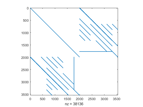
The matrix has 3,543 rows with some 38,136 nonzero elements, i.e., some 10 nonzero entries per row. Now the timing for Matlab's backslash and our sparse solver is as follows:

b = A*(2*rand(n,1)-1);
tic
xs = A\b;                   % approximation by Matlab's backslash
tbackslash = toc;
tic
Y = verifylss(A,b);         % verified inclusion using sparse solver
Tsparse = toc;
format short
timing = [tbackslash Tsparse]

relerrbackslash =
   1.5447e-15   1.6530e-11
relerrY =
   1.4751e-16   2.2200e-16

As can be seen the verified sparse solver requires only one fourth of the computing time of Matlab's backslash. Again we can judge the quality of the results using our verified error bounds :

format shorte
rxs = relerr(xs,Y);
relerrbackslash = [median(rxs) max(rxs)]
rSparse = relerr(Y);
relerrY = [median(rSparse) max(rSparse)]

Matlab's backslash has 15 correct digits in the median and at least 11 correct digits. There are examples where Matlab's backslash is slower than our verification algorithm by two orders of magnitudes - but also vice versa.

Methods for sparse matrices

For INTLAB Version 14 I derived two different methods for solving sparse linear systems, namely verifylssSparse1 based on

S.M. Rump: Verified error bounds for sparse systems Part I: The splitting of a matrix into two factors, to appear

and verifylssSparse2 based on

S.M. Rump: Verified error bounds for sparse systems Part II: Inertia-based bounds, least squares and nonlinear systems, to appear

A key point for both methods is factoring the matrix A into L1*L2 with triangular factors with the property that L1 and L2 have identical sets of singular values, and that the condition numbers of L1 (and of L2) are of size cond(A)^(1/2). Hence, a lower bound for the smallest singular values of L1 (and L2) can be computed using L1'*L1. That allows to treat matrices with condition number up to 1e16, the natural bound for computing in double precision (binary64).

Algorithm verifylssSparse1 is sometimes faster than verifylssSparse2, however, in few cases verifylssSparse2 is able to compute verified bounds but verifylssSparse1 cannot.

Because of the importance of sparse linear systems I put both algorithms verifylssSparse1 and verifylssSparse2 into INTLAB Version 14.

The general algorithm verifylss for linear systems has been adapted to check for sparsity of the matrix. As a consequence, verifylss calls the method as before for dense matrix, and as the default, it calls verifylssSparse1 for sparse input matrix.

A complex linear system and comparison verifylssSparse1 and 2

Consider example 326 of the Florida Sparse Matrix Collection

Problem = ssget(326)
A = Problem.A;
n = dim(A)
nnzA = nnz(A)
norm_imagA = norm(imag(A),inf)

Problem = 
  struct with fields:

     title: 'MODEL H2+ IN AN ELECTROMAGNETIC FIELD, S.I. CHU'
         A: [2534×2534 double]
      name: 'Bai/qc2534'
        id: 326
      date: '1991'
    author: 'S. Chu'
        ed: 'Z. Bai, D. Day, J. Demmel, J. Dongarra'
      kind: 'electromagnetics problem'
n =
        2534
nnzA =
      463360
norm_imagA =
   1.4915e-01

with 2,534 rows and 463,360 nonzero elements. The timing for verifylssSparse1 and verifylssSparse2 is as follows:

b = A*(2*rand(n,1)-1);
tic
[X1,delta1] = verifylssSparse1(A,b);     % verified inclusion using algorithm 1
T1 = toc;
tic
[X2,delta2] = verifylssSparse2(A,b);     % verified inclusion using algorithm 2
T2 = toc;
format short
timing = [T1 T2]

timing =
   12.4365   20.8511

As can be seen, verifylssSparse1 is significantly faster than verifylssSparse2. Both algorithms produce inclusions with maximal accuracy:

format shorte
r = delta1./abs(X1);
relerr1 = [median(r) max(r)]
r = delta2./abs(X2);
relerr2 = [median(r) max(r)]

relerr1 =
   3.8198e-17   1.1004e-16
relerr2 =
   3.8198e-17   1.1004e-16

A linear system with interval data

Consider example 2692 of the Florida Sparse Matrix Collection

Problem = ssget(2692)
A = Problem.A;
n = dim(A)
nnzA = nnz(A)

Problem = 
  struct with fields:

      name: 'VDOL/hangGlider_2'
     title: 'hangGlider optimal control problem (matrix 2 of 5)'
         A: [1647×1647 double]
         b: [1647×1 double]
        id: 2692
      date: '2015'
    author: 'B. Senses, A. Rao'
        ed: 'T. Davis'
      kind: 'optimal control problem'
     notes: [47×71 char]
       aux: [1×1 struct]
n =
        1647
nnzA =
       14754

with 1,647 rows and 14,754 nonzero elements, i.e., some 9 nonzero elements per row. The timing for Matlab's backslash and the full and the sparse solver is:

b = A*(2*rand(n,1)-1);
tic
xs = A\b;                   % approximation by Matlab's backslash
tbackslash = toc;
tic
X = verifylss(full(A),b);   % verified inclusion using full solver
Tfull = toc;
tic
Y = verifylss(A,b);         % verified inclusion using sparse solver
Tsparse = toc;
format short
timing = [tbackslash Tfull Tsparse]

timing =
    0.0146    0.7865    0.0544

As can be seen the sparse verification method is faster than the full method by an order of magnitude. The accuracy is as before, i.e., maximal accuracy:

format shorte
rxs = relerr(xs,Y);
relerrbackslash = [median(rxs) max(rxs)]
rX = relerr(X);
relerrX = [median(rX) max(rX)]
rSparse = relerr(Y);
relerrY = [median(rSparse) max(rSparse)]

relerrbackslash =
   3.2103e-14   9.0470e-09
relerrX =
   1.4718e-16   2.2184e-16
relerrY =
   1.4718e-16   2.2184e-16

Next we afflict the data of the matrix with tolerances. The condition number of A

condA = cond(full(A))

      e          time        median relative error
             full   sparse      full     sparse
---------------------------------------------------
  1.0e-16    0.59    0.07     9.5e-12   2.0e-04
  1.0e-14    0.58    0.03     1.8e-10   4.8e-03
  1.0e-12    0.63    0.03     1.7e-08   3.6e-01
  1.0e-10    0.62    0.03     1.7e-06   2.1e+01
  1.0e-08    0.60    0.03     1.7e-04   2.8e+03
  1.0e-06    0.62    0.07     1.6e-02       NaN
  1.0e-04    0.57    0.07     7.9e-01       NaN

suggests that for relative perturbations exceeding 1e-6 the interval matrix contains a singular matrix. We afflict the input matrix with a multiplicative tolerance 1 +/- e.

midA = A;
disp('      e          time        median relative error')
disp('             full   sparse      full     sparse')
disp('---------------------------------------------------')
for e=10.^[-16:2:-4]
  intA = midA.*midrad(1,e);
  tic
  X = verifylss(full(intA),b);   % verified inclusion using full solver
  Tfull = toc;
  tic
  Y = verifylss(intA,b);         % verified inclusion using sparse solver
  Tsparse = toc;
  fprintf('  %6.1e%8.2f%8.2f    %8.1e  %8.1e\n', ...
    e,Tfull,Tsparse,median(relerr(X)),median(relerr(Y)))
end

Again the sparse solver is much faster than the full solver, however, the full solver is significantly more accurate and can reach larger tolerances. For tolerance 1 +/- 1e-4 all matrices within the interval matrix intA are still regular, but even the full solver cannot succeed. That can also be verified by

isreg = isregular(intA)

isreg =
     1

The result 1 proves with mathematical certainty that all matrices within intA are regular; if the result would be 0 that fact could not be decided. Recall that checking regularity an NP-hard problem.

A problem where verifylssSparse1 fails but verifylssSparse2 is successful

Consider example 934 of the Florida Sparse Matrix Collection

Problem = ssget(934)
A = Problem.A;
n = dim(A)
nnzA = nnz(A)

Problem = 
  struct with fields:

         A: [7055×7055 double]
         b: [7055×1 double]
      name: 'Lucifora/cell1'
     title: 'Telecom Italia Mobile, GSM cell phone problem (cell1)'
        id: 934
     Zeros: [7055×7055 double]
      date: '2003'
    author: 'S. Lucifora'
        ed: 'T. Davis'
      kind: 'directed weighted graph'
n =
        7055
nnzA =
       30082

The matrix has 7,055 rows with somd 30,082 nonzero elements. Now the second algorithm verifylssSparse2 computes an inclusion successfully, but verifylssSparse1 fails:

b = A*(2*rand(n,1)-1);
tic
[X1,delta1] = verifylssSparse1(A,b);     % verified inclusion using algorithm 1
T1 = toc;
tic
[X2,delta2] = verifylssSparse2(A,b);     % verified inclusion using algorithm 2
T2 = toc;
format short
timing = [T1 T2]

timing =
    1.1654    1.1539

Algorithm verifylssSparse1 failed, indicated by NaN's, but the inclusions by verifylssSparse2 is maximally accurate:

format shorte
r = delta1./abs(X1);
relerr1 = [median(r) max(r)]
r = delta2./abs(X2);
relerr2 = [median(r) max(r)]

relerr1 =
   NaN   NaN
relerr2 =
   3.6735e-17   1.0920e-16

Equilibration may be counterproductive

Usually equilibration of the input matrix is beneficial. Often the condition number drops by several orders of magnitude. However, in rare cases equilibration is counterproductive.

Consider example 1210 of the Florida Sparse Matrix Collection

Problem = ssget(1210)
A = Problem.A;
n = dim(A)
nnzA = nnz(A)
condA = condest(A)

Problem = 
  struct with fields:

      name: 'Oberwolfach/t3dl_a'
     title: 'Oberwolfach: micropyros thruster, A matrix'
         A: [20360×20360 double]
        id: 1210
      kind: 'duplicate model reduction problem'
      date: '2004'
    author: 'E. Rudnyi'
        ed: 'E. Rudnyi'
n =
       20360
nnzA =
      509866
condA =
   8.0795e+14

with 20,360 unknowns and 509,866 nonzero elements. The estimated condition number is 8e14.

The sparse linear system solvers allow an extra parameter to switch equilibration off (the default is on). Next we test the two sparse solvers verifylssSparse1/2 with equilibration on/off:

b = A*randn(n,1);

res = [];
for equil=[true false]
  [xs,delta] = verifylssSparse1(A,b,equil);
  rel = delta./abs(xs);
  res = [res median(rel)];
end
disp(sprintf('verifylssSparse1     with equilibration  median(relerr) = %8.1e',res(1)))
disp(sprintf('                  without equilibration  median(relerr) = %8.1e',res(2)))
disp(' ')

res = [];
for equil=[true false]
  [xs,delta] = verifylssSparse2(A,b,equil);
  rel = delta./abs(xs);
  res = [res median(rel)];
end
disp(sprintf('verifylssSparse2     with equilibration  median(relerr) = %8.1e',res(1)))
disp(sprintf('                  without equilibration  median(relerr) = %8.1e',res(2)))
disp(' ')

verifylssSparse1     with equilibration  median(relerr) =      NaN
                  without equilibration  median(relerr) =  3.9e-17
 
verifylssSparse2     with equilibration  median(relerr) =  3.9e-17
                  without equilibration  median(relerr) =  3.9e-17

As can be seen, verifylssSparse1 succeeds without but fails with equilibration, whereas verifylssSparse2 succeeds with and without equilibration.

Note that the sparse nonlinear system solver verifynlssSparse accepts an extra parameter for switching equilibration off as well.

A least squares problem

Consider example 981 of the Florida Sparse Matrix Collection

Problem = ssget(981)
A = Problem.A;
[m n] = size(A)
nnzA = nnz(A)

timing =
   20.1142   10.9436

The matrix has 29,493 rows for a least squares problem with 11,822 unknowns. The matrix contains 117,954 nonzero elements.

format short
b = A*(2*rand(n,1)-1);
tic
xs = A\b;                       % approximation by Matlab's backslash
t = toc;
tic
X = verifylss(A,b);             % verified inclusion using sparse solver
T = toc;
timing = [t T]

Here verification is again significantly faster than the computation of an approximation by Matlab's backslash algorithm. The accuracy is as follows:

format shorte
rxs = relerr(xs,X);
relerrbackslash = [median(rxs) max(rxs)]
rX = relerr(X);
relerrX = [median(rX) max(rX)]

relerrbackslash =
   3.6586e-12   1.3424e-07
relerrX =
   1.4851e-16   2.2204e-16

Matlab's backslash produces some 12 correct digits in the median but also only 8 correct digits for some entries. Our verified bounds are maximally accurate for all entries of the result.

Underdetermined linear systems

For underdetermined linear systems for a matrix with m rows and n unknowns, m<n, Matlab chooses to compute a minimum norm solution with at most m nonzero elements. We took the following example from Matlab's documentation of the backslash operator (mldivide):

format short
A = [1 2 0; 0 4 3];
b = [8; 18];
x = A\b

In contrast we choose to compute an inclusion of the minimum 2-norm solution, i.e., P*b for P denoting the pseudoinverse of A:

format long _
X = verifylss(A,b)
P = pinv(intval(A));
Xpinv = P*b
format short

intval X = 
   0.91803278688524
   3.54098360655737
   1.27868852459016
intval Xpinv = 
   0.91803278688525
   3.54098360655737
   1.27868852459016

The latter method, multiplying the right hand side by an inclusion of the pseudoinverse, should definitely not be used, it is just displayed for demonstration purposes.

Indeed, the 2-norm of the inclusion X is smaller than that of Matlab's x:

normx = norm(x)
normX = norm(X)

normx =
    4.0552
intval normX = 
    3.8751

Both inclusions X and Xpinv are maximally accurate, however, the first component is not the same. To verify that both results are correct we use the Advanpix multiple precision toolbox:

mp.Digits(34);
Xmp = mp(A)\b

Xmp = 
        0.9180327868852459016393442622950817    
         3.540983606557377049180327868852459    
         1.278688524590163934426229508196722

Recall that subtracting and adding 1 to the last displayed digit in the underscore format is a correct inclusion. Thus, both inclusions X and Xpinv are correct.

Because of the different results we cannot compare the results and performance of our verification methods with Matlab's backslash approximation.

To give one example, consider example 1948 of the Florida Sparse Matrix Collection

Problem = ssget(1948)
A = Problem.A;
[m n] = size(A)
nnzA = nnz(A)

Problem = 
  struct with fields:

      name: 'JGD_Forest/TF14'
     title: 'Forests and Trees from Nicolas Thiery'
         A: [2644×3160 double]
        id: 1948
      date: '2008'
    author: 'N. Thiery'
        ed: 'J.-G. Dumas'
      kind: 'combinatorial problem'
     notes: [16×60 char]
m =
        2644
n =
        3160
nnzA =
       29862

with 2,644 rows for 3,160 unknowns.

format short
b = A*(2*rand(n,1)-1);
tic
X = verifylss(A,b);         % verified inclusion using sparse solver
T = toc

format shorte
rX = relerr(X);
relerrbackslash = [median(rX) max(rX)]

As can be seen the inclusions for all entries is about maximally accurate.

Systems of nonlinear equations

Consider the following example:

Abbot/Brent     3 y" y + y'^2 = 0;    y(0)=0; y(1)=20;
approximation   10*ones(n,1)
solution        20*x^.75
y = x;
n = length(x); v=2:n-1;
y(1) = 3*x(1)*(x(2)-2*x(1)) + x(2)*x(2)/4;
y(v) = 3*x(v).*(x(v+1)-2*x(v)+x(v-1)) + (x(v+1)-x(v-1)).^2/4;
y(n) = 3*x(n).*(20-2*x(n)+x(n-1)) + (20-x(n-1)).^2/4;

The number of unknowns can be specified, the initial approximation is the vectors of all 10's. Following we choose n = 3000 unknowns.

format short
n = 3000;
xs = 10*ones(n,1);

The gradient toolbox (as well as the Hessian toolbox) allow to specify a threshold of the number of unknowns from where gradients (or Hessians) are treated as sparse. More precisely, sparsegradient(m) specifies that gradients with at least m unknowns are treated sparse. As a consequence, sparsegradient(inf) forces to treat gradients always full.

To solve a nonlinear system with sparse gradients, we can either use sparsegradient(0) and verifynlss, or directly verifynlssSparse.

We apply the to the nonlinear system above:

sparsegradient(inf);    % gradient always full
tic
Xfull = verifynlss(@test,xs);
tfull = toc;

tic
Xsparse = verifynlssSparse(@test,xs);
tsparse = toc;

timing = [tfull tsparse]

format shorte
r = relerr(Xfull);
relerrfull = [median(r) max(r)]
r = relerr(Xsparse);
rererrsparse = [median(r) max(r)]

===> Gradient derivative always stored full
timing =
    8.6779    0.4900
relerrfull =
   1.0625e-16   4.3735e-16
rererrsparse =
   1.8677e-12   9.7428e-10

As can be seen, treating the nonlinear system with full Jacobian needs about 20 times as much computing time than with sparse Jacobian. The full solver achieves maximal accuracy, the sparse solver guarantees some 12 decimal digits in the median, at least 9 digits.

The sparse nonlinear solver requires the solution of a linear system with the Jacobian matrix and an interval right hand side for some interval iteration. That causes quite some overestimation so that for too large number of unknowns the method fails.

n = 4000;
xs = 10*ones(n,1);

format short
tic
Xsparse = verifynlssSparse(@test,xs);  % using the default verifylssSparse1
tsparse = toc
Xsparse(1)

tsparse =
    0.5403
intval ans = 
       NaN

The sparse nonlinear system solver needs to solve a sparse linear system. To that end there is a choice of two methods: verifylssSparse1 (default) and verifylssSparse2. The latter succeeds to compute an inclusion of our sample nonlinear system for n = 4000, but fails as well for n = 5000:

n = 4000;
xs = 10*ones(n,1);
format short
tic
Xsparse4000 = verifynlssSparse(@test,xs,2); % using verifylssSparse2
tsparse = toc
format long
Xsparse4000(1)

n = 5000;
xs = 10*ones(n,1);
format short
tic
Xsparse5000 = verifynlssSparse(@test,xs,2); % using verifylssSparse2
tsparse = toc
format long
Xsparse5000(1)
format short

tsparse =
    0.4813
intval ans = 
   0.0367272736____
tsparse =
    0.8176
intval ans = 
                NaN

The full solver is based on a different method and very stable. It is much slower

sparsegradient(inf);    % gradient always full
tic
Xfull = verifynlss(@test,xs);
tfull = toc
format shorte
r = relerr(Xfull);
relerrfull = [median(r) max(r)]

===> Gradient derivative always stored full
tfull =
   27.6849
relerrfull =
   1.0584e-16   4.6557e-16

but succeeds to compute a verified inclusion with almost maximal accuracy.

Local minumum of a function f:R^n->R

A sufficiently smooth function f:R^n->R has a stationary point if, and only if, its gradient is zero. That means to solve a system of nonlinear equations in n unknowns. The function has a local minimum at that solution if the Hessian is positive definite. Consider

Source: Problem 61 in
A.R. Conn, N.I.M. Gould, M. Lescrenier and Ph.L. Toint,
"Performance of a multifrontal scheme for partially separable
optimization",
Report 88/4, Dept of Mathematics, FUNDP (Namur, B), 1988.

SIF input: Ph. Toint, Dec 1989.
classification SUR2-AN-V-0

param N:=1000; var x{1..N} := 1.0;

minimize f: sum {i in 1..N-4} (-4*x[i]+3.0)^2 + sum {i in 1..N-4} (x[i]^2+2*x[i+1]^2+3*x[i+2]^2+4*x[i+3]^2+5*x[N]^2)^2;

The call y = test_h(x,2) computes the function value at x in R^n. The initial approximation is ones(n,1).

The Jacobian of the nonlinear system to find an inclusion of f'(x)=0 is the Hessian of f. The statement sparsehessian(k) controls that Hessians are stored sparse for at least k unkowns. Consequently, sparsehessian(inf) stores Hessians always full, whereas sparsehessian(0) stores Hessians always sparse.

After finding an inclusion X of a stationary point of f we use INTLAB's isspd to verify that the Hessian of f for every x in X is positive definite. That includes the stationary point which is therefore proved to be a local minimum.

Following we compare finding a local minimum with full and with sparse Hessian for n=200 unknowns:

n = 200;
sparsehessian(inf);
tic
Xfull = verifylocalmin(@test_h,ones(n,1),0,2);
tfull = toc;
sparsehessian(0);
tic
Xsparse = verifylocalmin(@test_h,ones(n,1),0,2);
tsparse = toc;
format short
timing = [tfull tsparse]

===> Hessian derivatives always stored full
===> Hessian derivatives always stored sparse
timing =
   22.4948    0.1942

As can be seen the sparse solver is some 50 times faster than the full solver for n=200. The maximum relative error is as follows:

relerrfull = max(relerr(Xfull))
relerrsparse = max(relerr(Xsparse))

relerrfull =
   5.8244e-16
relerrsparse =
   1.6957e-13

The inclusion by the full solver is maximally accurate, that of the sparse solver guarantees at least 13 correct digits.

Following we consider the same example with larger number of unknowns:

for n=[1000 2000 5000 10000]
  tic
  Xsparse = verifylocalmin(@test_h,ones(n,1),0,2);
  tsparse = toc;
  relerrSparse = max(relerr(Xsparse));
  fprintf('n=%6d, time %4.1f seconds, maximum relative error %7.1e\n',n,tsparse,relerrSparse)
end

For n = 10,000 unknowns the computing time is a little more than 1 minute and guarantees at least 12 correct digits for each entry.

Enjoy INTLAB

INTLAB was designed and written by S.M. Rump, head of the Institute for Reliable Computing, Hamburg University of Technology. Suggestions are always welcome to rump (at) tuhh.de