DEMOINTLAB_RESIDUALS Fast and accurate matrix residuals

The accurate computation of residuals is the key to compute accurate inclusions of the solution of a system of linear or nonlinear equations.

Two new algorithms prodK and spProdK
Residuals
Accurate residuals
Accurate inclusion of residuals
Performance of prodK
Performance of prodK versus mp of Advanpix
Performance improvement using Karatsuba's method
Results represented by an unevaluated sum
Inversion of extremely ill-conditioned matrices in double precision
Residuals with sparse data
Performance of spProdK versus mp of Advanpix for sparse data
Enjoy INTLAB

Two new algorithms prodK and spProdK

From INTLAB Version 14 new and versatile algorithms to compute approximations and/or verified bounds for matrix residuals are included. They supersede previous algorithms such as AccDot, Dot_, Dot2, Dot2_, DotK, and others, see the demo file 'daccsumdot' (Accurate summation and dot products). The old routines are left in INTLAB for upward compatibility.

Two new algorithms are added, namely prodK for full input and spProdK for sparse input. The algorithms are based on

M. Lange and S.M. Rump: Accurate floating-point matrix products, to appear

and the superb implementation of both algorithm is due to Marko Lange. The algorithms are very fast although entirely implemented in Matlab/Octave - as all algorithms in INTLAB. My dearest thanks to Marko for these outstanding algorithms.

Residuals

The accurate approximation and inclusion of residuals is mandotory and ubiquitous to compute verified bounds successfully and accurately. A typical example are verified bounds for the solution of a linear system. Consider

setround(0)         % rounding to nearest
format short

n = 1000
A = randmat(n,1e12);
cnd = cond(A)
b = A*ones(n,1);

n =
        1000
cnd =
   1.0000e+12

A random matrix with anticipated condition number cnd = 1e12 is generated together with a right hand side such that the solution of the linear system Ax=b is close to all 1's. We first compute an inclusion of A^-1 b by our standard algorithm verifylss:

X = verifylss(A,b);

The inclusion X is close to maximally accurate:

rel = relerr(X);
relX = [median(rel) max(rel)]

relX =
   1.0e-15 *
    0.1110    0.2221

The approximation by Matlab's backslash

xs = A\b;
rel = relerr(xs,X);
relxs = [median(rel) max(rel)]

relxs =
   1.0e-03 *
    0.0042    0.1544

is correct to 5 digits in the median and 3-4 digits in the worst case - as expected from the condition number. The classical residual iteration, i.e., Newton method, should improve the accuracy of xs:

for k=1:2
  xs = xs - A\(A*xs-b);
  rel = relerr(xs,X);
  relxs = [median(rel) max(rel)]
end

relxs =
   1.0e-04 *
    0.0108    0.3924
relxs =
   1.0e-04 *
    0.0066    0.2680

Accurate residuals

As is well known Skeel proved that one residual iteration in working precision ensures backward stability, however, the accuracy of the approximation is only improved when calculating the residual in some higher precision. That is done by prodK:

for k=1:3
  xs = xs - A\prodK(A,xs,-1,b,2);
  rel = relerr(xs,X);
  relxs = [median(rel) max(rel)]
end

relxs =
   1.0e-09 *
    0.0044    0.2315
relxs =
   1.0e-14 *
    0.0222    0.1110
relxs =
   1.0e-15 *
    0.1110    0.4441

As can be seen three residual iterations suffice for an approximation with maximal accuracy. The syntax of algorithm prodK is

r = prodK(a1,b1,a2,b2,...,am,bm,k)

with m>=1. The input pairs may be real or complex.

The pair products ai*bi must all have equal dimension pxq for i=1..m. An exeption is that the first factor ai may be scalar in which case bi is of dimension pxq.

The final input parameter k specifies that the computation is 'as if' computed in (k/2+1)-fold precision. That means for k=2 as above the result is as computed in extended precision, for k=4 as if in 3-fold precision, and so forth.

A typical application is the matrix residual with respect to an approximate inverse:

R = inv(A);
C = prodK(R,A,-1,eye(n),2);
maxC = max(abs(C(:)))

maxC =
   1.1247e-04

The residual is small, however, that is an approximation, not inclusion of the residual.

Accurate inclusion of residuals

An inclusion uses the same syntax as before except that there is a second output parameter for the error:

[r,e] = prodK(a1,b1,a2,b2,...,am,bm,k)

It follows that the true product P := sum(i=1..m,ai*bi) satisfies

r - e  <= P <= r + e .

An application to the matrix residual is

[C,E] = prodK(R,A,-1,eye(n),2);
setround(1)
normRes = norm(abs(C)+E,inf)
setround(0)

normRes =
    0.0027

It follows that the inf-norm of the residual RA-I is strictly less than 1 so that RA-I is convergent and both R and A are nonsingular.

Performance of prodK

Because of its importance we offered previously several dot product routines, for example Dot2_ with the similar syntax

P = Dot2_(A1,B1,A2,B2,...)

On return, P is an inclusion of A1*B1 + A2+B2 + ... with accuracy as if computed in 2-fold precision. The input maybe real or complex. The computational precision is the same as of prodK for k=2, so we can compare the performance directly, first for matrix-vector multiplication:

N = [10 30 100 300 1000 3000 10000];
tDot2_ = zeros(1,length(N));
tprodK = zeros(1,length(N));
for i=1:length(N)
  n = N(i);
  A1 = randn(n);
  B1 = randn(n,1);
  A2 = randn(n);
  B2 = randn(n,1);
  tic
  C = Dot2_(A1,B1,A2,B2);
  tDot2_(i) = toc;
  tic
  [C,E] = prodK(A1,B1,A2,B2,2);
  tprodK(i) = toc;
end
disp(sprintf('matrix*vector   n %6d%6d%6d%6d%6d%6d%6d',N))
disp(repmat('-',1,60))
disp(sprintf('t(Dot2_)/t(prodK) %6.1f%6.1f%6.1f%6.1f%6.1f%6.1f%6.1f',tDot2_./tprodK))

matrix*vector   n     10    30   100   300  1000  3000 10000
------------------------------------------------------------
t(Dot2_)/t(prodK)    0.7   2.0   4.7   6.9   2.0   0.9   0.8

Here both Dot2_ and prodK compute inclusions of the true result.

We display the time ratio t(Dot2_)/t(prodK), i.e., a ratio 2 means that the new prodK is twice as fast as Dot2_. For medium size dimensions the new prodK is faster than Dot2_, for large vector length Dot2_ is faster. That changes for matrix multiplications:

N = [10 30 100 300 1000];
tDot2_ = zeros(1,length(N));
tprodK = zeros(1,length(N));
for i=1:length(N)
  n = N(i);
  A1 = randn(n);
  B1 = randn(n);
  A2 = randn(n);
  B2 = randn(n);
  tic
  C = Dot2_(A1,B1,A2,B2);
  tDot2_(i) = toc;
  tic
  [C,E] = prodK(A1,B1,A2,B2,2);
  tprodK(i) = toc;
end
disp(sprintf('matrix*matrix   n %6d%6d%6d%6d%6d',N))
disp(repmat('-',1,50))
disp(sprintf('t(Dot2_)/t(prodK) %6.1f%6.1f%6.1f%6.1f%6.1f',tDot2_./tprodK))

matrix*matrix   n     10    30   100   300  1000
--------------------------------------------------
t(Dot2_)/t(prodK)    0.9   2.7  14.7  25.0 130.5

With growing dimension the new prodK becomes increasingly faster than Dot2_. That is similar for complex data:

N = [10 30 100 300 1000];
tDot2_ = zeros(1,length(N));
tprodK = zeros(1,length(N));
for i=1:length(N)
  n = N(i);
  A1 = randomc(n);
  B1 = randomc(n);
  A2 = randomc(n);
  B2 = randomc(n);
  tic
  C = Dot2_(A1,B1,A2,B2);
  tDot2_(i) = toc;
  tic
  [C,E] = prodK(A1,B1,A2,B2,2);
  tprodK(i) = toc;
end
disp(sprintf('complex matrix  n %6d%6d%6d%6d%6d',N))
disp(repmat('-',1,50))
disp(sprintf('t(Dot2_)/t(prodK) %6.1f%6.1f%6.1f%6.1f%6.1f',tDot2_./tprodK))

complex matrix  n     10    30   100   300  1000
--------------------------------------------------
t(Dot2_)/t(prodK)    0.9   3.9  14.1  37.3 102.5

Performance of prodK versus mp of Advanpix

Another possibility to calculate accurate approximations of residuals is using the multiple precision package by Advanpix. Here the computing precision can be freely defined. A particular fast implemention uses mp.Digits(34) corresponding to extended precision according to the IEEE754 arithmetic standard. The operations respect the rounding mode.

The mp-toolbox in Advanpix is written in highly optimized C-code whereas INTLAB is entirely written in Matlab/Octave suffering from interpretation overhead. Nevertheless we compare the performance of Advanpix and prodK, first for matrix-vector multiplication:

N = [10 30 100 300 1000 3000 10000];
tmp = zeros(1,length(N));
tprodK = zeros(1,length(N));
mp.Digits(34);
for i=1:length(N)
  n = N(i);
  A1 = randn(n);
  B1 = randn(n,1);
  A2 = randn(n);
  B2 = randn(n,1);
  tic
  double(mp(A1)*B1+mp(A2)*B2);
  tmp(i) = toc;
  tic
  prodK(A1,B1,A2,B2,2);
  tprodK(i) = toc;
end
disp(sprintf('matrix*vector  n %6d%6d%6d%6d%6d%6d%6d',N))
disp(repmat('-',1,60))
disp(sprintf('t(mp)/t(prodK)   %6.1f%6.1f%6.1f%6.1f%6.1f%6.1f%6.1f',tmp./tprodK))

matrix*vector  n     10    30   100   300  1000  3000 10000
------------------------------------------------------------
t(mp)/t(prodK)      1.3   1.0   1.7   4.1   2.3   1.8   1.8

Both mp in mp.Digits(34) as prodK with k=2 compute approximations as if computed in extended precision.

Despite the interpretation overhead the new prodK is often twice as fast as mp by Advanpix. Following is a similar test for matrix-matrix multiplication.

N = [10 30 100 300 1000];
tmp = zeros(1,length(N));
tprodK = zeros(1,length(N));
mp.Digits(34);
for i=1:length(N)
  n = N(i);
  A1 = randn(n);
  B1 = randn(n);
  A2 = randn(n);
  B2 = randn(n);
  tic
  double(mp(A1)*B1+mp(A2)*B2);
  tmp(i) = toc;
  tic
  prodK(A1,B1,A2,B2,2);
  tprodK(i) = toc;
end
disp(sprintf('matrix*matrix  n %6d%6d%6d%6d%6d',N))
disp(repmat('-',1,60))
disp(sprintf('t(mp)/t(prodK)   %6.1f%6.1f%6.1f%6.1f%6.1f',tmp./tprodK))

matrix*matrix  n     10    30   100   300  1000
------------------------------------------------------------
t(mp)/t(prodK)      0.7   1.9   9.3  36.1  55.9

Now for larger dimensions the new prodK becomes significantly faster than Andvanpix' mp.

Since Advanpix in mp.Digits(34) corresponding to extended precision respects the rounding mode, it is also possible to compute verified inclusions. Following is an example of matrix-matrix products:

N = [10 30 100 300 1000];
tmp = zeros(1,length(N));
tprodK = zeros(1,length(N));
mp.Digits(34);
for i=1:length(N)
  n = N(i);
  A1 = randn(n);
  B1 = randn(n);
  A2 = randn(n);
  B2 = randn(n);
  tic
  setround(-1)
  Cdown = double(mp(A1)*B1+mp(A2)*B2);
  setround(1)
  Cup = double(mp(A1)*B1+mp(A2)*B2);
  setround(0)
  tmp(i) = toc;
  tic
  [C,E] = prodK(A1,B1,A2,B2,2);
  tprodK(i) = toc;
end
disp(sprintf('matrix*matrix  n %6d%6d%6d%6d%6d',N))
disp(repmat('-',1,60))
disp(sprintf('t(mp)/t(prodK)   %6.1f%6.1f%6.1f%6.1f%6.1f',tmp./tprodK))

matrix*matrix  n     10    30   100   300  1000
------------------------------------------------------------
t(mp)/t(prodK)     25.2   4.8  17.4  73.3 115.3

As can be seen our prodK is significantly faster than mp despite interpretation overhead. Note that the mp-toolbox needs two calls in rounding downwards and upwards, whereas for prodK one call with the extra output argument E for the error is sufficient.

Performance improvement using Karatsuba's method

For matrix with larger dimension prodK uses Karatruba's method. The threshold for k=2 is n=333. The effect can be seen as follows:

for n=333:334
  A = randn(n);
  tic
  prodK(A,A,2);
  toc
end

Elapsed time is 0.010094 seconds.
Elapsed time is 0.005960 seconds.

For n=334 prodK switches to Karatsuba's method with some gain in computing time.

Results represented by an unevaluated sum

A higher precision may be simulated by an unevaluated sum. Consider the algorithm InvIllco (which is included in INTLAB) from

S.M. Rump: Inversion of extremely ill-conditioned matrices in floating-point,
  Japan J. Indust. Appl. Math. (JJIAM), 26:249-277, 2009.

It shows how to invert extremely ill-conditioned matrices in working precision, i.e., double precision (binary64). We first generate a very ill-conditioned random matrix.

n = 50;
A = randmat(n,1e25);    % random matrix with cond(A)~1e25
R = inv(A);             % no digit is correct
mp.Digits(34);
Rmp = double(inv(mp(A)));
v = 1:5;
Rv = R(v,v)
Rmpv = Rmp(v,v)

Warning: Matrix is close to singular or badly scaled. Results may be inaccurate.
RCOND =  1.785061e-19. 
Rv =
   1.0e+14 *
   -2.2109   -2.5427    0.5260   -1.2500    1.2251
    2.3336    2.7120   -0.5425    1.3232   -1.2989
    2.4497    2.8248   -0.5794    1.3861   -1.3589
   -1.9765   -2.2807    0.4668   -1.1185    1.0968
   -0.4596   -0.5352    0.1063   -0.2607    0.2560
Rmpv =
   1.0e+19 *
    1.9780    2.2664   -0.4744    1.1172   -1.0943
   -2.0846   -2.3885    0.5000   -1.1774    1.1533
   -2.1908   -2.5102    0.5254   -1.2374    1.2120
    1.7675    2.0251   -0.4239    0.9983   -0.9778
    0.4104    0.4703   -0.0984    0.2318   -0.2271

As can be seen the approximate "inverse" R computed by Matlab's inv is off by 5 orders of magnitude, and often the sign is not correct. Nevertheless it has been shown in the paper above that R contains some useful information:

k = 2;
P = prodK(R,A,k);       % accurate product R*A
condP = cond(P)

condP =
   1.3542e+08

In the second line we use R as a preconditioner. Although it is off by orders of magnitude from the true inverse, the condition number of P drops by about the relative rounding error unit u~1e-16. Hence an approximate inverse X of P should be correct to about 7 digits.

X = inv(P);             % Matlab's approximate inverse

The call

r = prodK(a1,b1,a2,b2,...,am,bm,'OutputTerms',p,k)

specifies that the result is stored in a cell array r with p terms. Similarly,

[r,e] = prodK(a1,b1,a2,b2,...,am,bm,'OutputTerms',p,k)

stores an approximation to the result Res := sum(i=1..m,ai*bi) in the cell array r together with an error term e such that

| sum(i=1..p,r{i}) - Res | <= e .

Using X from above we compute an approximate inverse of the very ill-conditioned matrix A as follows:

R2 = prodK(X,R,k,'OutputTerms',k)  % new approximate inverse stored in k=2 terms

R2 =
  1×2 cell array
    {50×50 double}    {50×50 double}

We multiplied X by R and store the result as an unevaluated sum R{1}+R{2} of 2 matrices. The product is calculated with k=2, i.e., (k/2+1) = 2-fold precision, and the number of output terms is k=2, i.e., R2 is a cell array with 2 elements as well.

In theory XR = (RA)^-1 R = A^-1 R^-1 R = A^-1. And indeed using R{1}+R{2} as a preconditioner works well, extracting the hidden information Matlab's inverse:

P2 = prodK(R2,A,2);
rel = relerr(P2,eye(n));
format shorte
[median(rel(:)) max(rel(:))]
format short

ans =
   2.2737e-13   9.3132e-09

Note that in the first line the first parameter is R2, i.e., the unevaluated sum R{1}+R{2}. We can use R2 directly in prodK as parameter. The result P2 is R{1}*A + R{2}*A computed in 2-fold precision.

Together with prodK the approximate inverse R{1}+R{2} can be used to solve a linear system as well.

Inversion of extremely ill-conditioned matrices in double precision

It is shown in the paper above that this method can be iterated into an unevaluated sum of more than 2 summands. To that end we construct an extremely ill-conditioned matrix:

n = 50;
A = randmat(n,1e250);   % random matrix with cond(A)~1e250

We used

S.M. Rump: A Class of Arbitrarily Ill-conditioned Floating-Point Matrices,
  SIAM Journal on Matrix Analysis and Applications (SIMAX, 12(4):645-653, 1991.

to construct such an extremely ill-conditioned matrix.

The condition number cond(A)~1e250 implies that changing the input matrix A in the 250-th digit, the entries of its inverse change in the first place. As indicated by the mp-toolbox the true condition is even larger. Again we use the mp-toolbox with high precision to judge Matlab's approximate inverse R:

warning on
R = inv(A);                 % off by 260 orders of magnitude from A^-1
mp.Digits(300);             % using 300 digits precision
condAmp = double(cond(mp(A)))
Rmp = double(inv(mp(A)));   % inverse using 300 digits precision
v = 1:5;
Rv = R(v,v)
Rmpv = Rmp(v,v)

Warning: Matrix is close to singular or badly scaled. Results may be inaccurate.
RCOND =  2.009574e-19. 
condAmp =
  6.5868e+279
Rv =
   1.0e+05 *
    1.1142    0.5449   -0.0505    0.7622    0.0146
   -1.9961   -1.1933   -0.8453   -1.0174   -0.6411
   -1.3334   -0.9803   -1.3545   -0.3858   -0.9471
    2.8267    1.5298    0.5069    1.6976    0.4543
    5.0446    2.6119    0.3952    3.2191    0.4761
Rmpv =
  1.0e+267 *
   -0.5033   -0.3789   -0.5498   -0.1313   -0.3828
    0.1029    0.0775    0.1124    0.0268    0.0783
   -0.6053   -0.4558   -0.6613   -0.1579   -0.4605
   -0.7348   -0.5533   -0.8028   -0.1917   -0.5590
   -1.7462   -1.3148   -1.9076   -0.4554   -1.3283

Matlab's warning about a condition number is a little bit underestimated.

Matlab's approximate inverse R is off by some 260 orders of magnitude. Nevertheless the ratio between its entries is important and contains useful information. This is unveiled by the following code:

k = 1;
wng = warning;
warning off
tic
while norm(prodK(R,A,-1,eye(n),2*k-1),inf) > 1e-12
  k = k+1;
  P = prodK(R,A,2*k-1);
  X = inv(P);
  R = prodK(X,R,2*k-1,'OutputTerms',k);
end
time = toc
warning(wng)
R
norm(prodK(R,A,-1,eye(n),2*k-1),inf)

time =
    0.2625
R =
  1×19 cell array
  Columns 1 through 4
    {50×50 double}    {50×50 double}    {50×50 double}    {50×50 double}
  Columns 5 through 8
    {50×50 double}    {50×50 double}    {50×50 double}    {50×50 double}
  Columns 9 through 12
    {50×50 double}    {50×50 double}    {50×50 double}    {50×50 double}
  Columns 13 through 16
    {50×50 double}    {50×50 double}    {50×50 double}    {50×50 double}
  Columns 17 through 19
    {50×50 double}    {50×50 double}    {50×50 double}
ans =
   9.3674e-16

The iteration produces an approximate inverse R stored in 20 unevaluated terms. As a preconditioner it produces RA equal to the identity matrix with an error close to u~1e-16.

The implemention is particularly clear because the unevaluated sum can be used directly as parameter of prodK.

Moreover the computing time is less than half a second. We mention that the previous implementation of InvIllco in Version 13 of INTLAB used ProdKL and needed more than 2 minutes.

Residuals with sparse data

In principle prodK can be used for sparse matrices as well, however, the time penalty can be very large. To that end Marko Lange implemented a special version spProdK for sparse input. We offer both routines separately rather than automizing to leave the choice to the user.

The syntax is as of prodK:

r = spProdK(a1,b1,a2,b2,...,am,bm,k)

for an approximation r of the true product P := sum(i=1..m,ai*bi), and

[r,e] = spProdK(a1,b1,a2,b2,...,am,bm,k)

for an inclusion r - e <= P <= r + e.

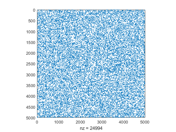
We generate a matrix of dimension 5000 with some 0.1 percent density.

n = 5000;
A = sprand(n,n,0.001);
close
spy(A)

The timing for prodK and spProdK is as follows:

tic
prodK(A,A,2);
tprodK = toc
tic
spProdK(A,A,2);
tspProdK = toc

tprodK =
    8.2638
tspProdK =
    0.0703

As can be seen the sparse version spProdK is faster by 2 orders of magnitude than prodK.

Performance of spProdK versus mp of Advanpix for sparse data

We also compare to the mp-toolbox using extended precision:

N = [1000 3000 10000 30000];
tmp = zeros(1,length(N));
tspProdK = zeros(1,length(N));
mp.Digits(34);
for i=1:length(N)
  n = N(i);
  A = sprand(n,n,0.001);
  tic
  double(mp(A)*A-A);
  tmp(i) = toc;
  tic
  spProdK(A,A,-1,A,2);
  tspProdK(i) = toc;
end
disp(sprintf('matrix*matrix  n   %6d%6d%6d%6d%6d',N))
disp(repmat('-',1,60))
disp(sprintf('t(mp)/t(spProdK)   %6.1f%6.1f%6.1f%6.1f%6.1f',tmp./tspProdK))

matrix*matrix  n     1000  3000 10000 30000
------------------------------------------------------------
t(mp)/t(spProdK)      0.1   1.3   1.9   1.6

As can be seen the highly optimized C-code in the Advanpix toolbox is for small dimensions faster than Marko Lange's Matlab/Octave code spProdK, for larger dimension spProdK outperforms the mp-toolbox.

The mp-toolbox with mp.Digits(34) corresponding to extended precision respects the rounding mode, however, two multiplications are necessary to compute the bounds.

N = [1000 3000 10000 30000];
tmp = zeros(1,length(N));
tprodK = zeros(1,length(N));
mp.Digits(34);
for i=1:length(N)
  n = N(i);
  A = sprand(n,n,0.001);
  tic
  setround(-1)
  Cdown = double(mp(A)*A-A);
  setround(1)
  Cup = double(mp(A)*A-A);
  setround(0)
  tmp(i) = toc;
  tic
  [C,E] = spProdK(A,A,-1,A,2);
  tspProdK(i) = toc;
end
disp(sprintf('matrix*matrix  n   %6d%6d%6d%6d%6d',N))
disp(repmat('-',1,60))
disp(sprintf('t(mp)/t(spProdK)   %6.1f%6.1f%6.1f%6.1f%6.1f',tmp./tspProdK))

matrix*matrix  n     1000  3000 10000 30000
------------------------------------------------------------
t(mp)/t(spProdK)      0.8   1.2   1.4   1.4

As can be seen the situation is very similar as before, for reasonable dimensions spProdK is faster than Advanpix' mp toolbox.

Enjoy INTLAB

INTLAB was designed and written by S.M. Rump, head of the Institute for Reliable Computing, Hamburg University of Technology. Suggestions are always welcome to rump (at) tuhh.de