DEMOPAIR A demonstration of CPair and Double-Double Arithmetic
Contents
- Pair arithmetic
- Initialization
- Display
- Performance comparison
- Accuracy of double-double and cpair arithmetic
- A typical cancellation
- A famous example I
- A famous example II
- Rigorous error bounds by the cpair arithmetic
-
Is Matlab's constant pi less than or larger than
 ?
?
- Inversion of very ill-conditioned matrices
- The residual of a matrix
- Polynomial evaluation I
- Polynomial evaluation II
- Polynomial evaluation III
- Least squares interpolation
- Plotting a polynomial near its roots: The Wilkinson polynomial
- Two-term recurrences, Muller's famous example
- Two-term recurrences, revisited
- Enjoy INTLAB
Pair arithmetic
Pair arithmetic increases the precision by storing pairs of numbers, the unevaluated sum of which is regarded as the result. The idea goes at least back to Dekker's 1971 paper "A Floating-Point Technique for Extending the Available Precision" in Numerische Mathematik.
A key ingredient are so-called error-free transformations. For example, for two floating-point numbers a,b a result x,y can be computed such that a+b=x+y or a*b=x+y and x is equal to the rounded-to-nearest result.
There are two toolboxes in INTLAB for a pair arithmetic, the well-known double-double arithmetic "dd" and a new "cpair" based on
M. Lange and S.M. Rump. Faithfully Rounded Floating-point Computations.
   ACM transactions on mathematical software, 46(3), 2020.
A simple example is as follows:
format short cpairDouble ddDouble   % short display for floating-point, pairs as double
setround(0)                         % rounding to nearest
e = 1e-25;
x = ( 1 + e ) - 1
E1 = cpair(e);  X1 = ( 1 + E1 ) - 1
E2 = dd(e);     X2 = ( 1 + E2 ) - 1
===> Cpair display of .hi + .lo as double
===> Double-double display of .hi + .lo as double
x =
     0
cpair-type X1 =
   1.0000e-25
dd-type X2 =
   1.0000e-25
The value of e is too small to be captured by ordinary binary64 floating-point arithmetic; both pair arithmetics yield the correct answer.
The comparison in flops between double-double and cpair arithmetic is as follows:
      dble+pair pair+pair  dble.*pair  pair.*pair  sqr(pair)
cpair        8       9          19          22         20
   dd       10      18          21          24         23
      dble/pair  pair/dble  pair/pair  sqrt(pair)
cpair       24       22         25          23
   dd       32       25         33         100
Moreover, our cpair system allows for a complete error analysis, i.e., when A is computed in cpair arithmetic, then errbound(A) bounds the true error of the result. In contrast to double-double, the high order part of a cpair result is equal to the result of ordinary floating-point arithmetic, i.e., the lower order part is a correction term.
Initialization
Floating-point quantities become double-double or cpair by a standard type cast:
A = -3.5
B = 17
ddAB = dd(A)/B
cpairAB = cpair(A)/B
A =
   -3.5000
B =
    17
dd-type ddAB =
   -0.2059
cpair-type cpairAB =
   -0.2059
Display
There are several ways to display a double-double or a cpair result. Above the usual double format was used, however, that does not display the full accuracy. To see that use
format ddHiLo
ddAB
format cpairHiLo
cpairAB
===> Double-double display of .hi and .lo separately as double
dd-type ddAB.hi =
   -0.2059
dd ddAB.lo =
  -9.7961e-18
===> Cpair display of .hi and .lo separately as double
cpair-type cpairAB.hi =
   -0.2059
cpair-type cpairAB.lo =
  -9.7961e-18
or a long display to see all digits:
format ddLong
ddAB
format cpairLong
cpairAB
===> Double-double display of .hi + .lo as long column vector
dd-type ddAB =
 -2.058823529411764705882352940986401513 * 10^-0001
===> Cpair display of .hi + .lo as long column vector
cpair-type cpairAB =
 -2.058823529411764705882352940986401513 * 10^-0001
Performance comparison
The new cpair arithmetic needs fewer operations, and the time factor to double-double is even more favorite. Consider a 500x500 matrix:
n = 500;
K = 100;
a = randn(n);
cpairinit('WithoutErrorTerm')
===> Cpair computations without error terms, errbound(A) cannot be used
ans =
    'WithoutErrorTerm'
We first compare "pair op double" for two 1000x1000 matrices, 100 test cases each:
disp('pair op double:')
disp(' ')
fprintf('      op           t_dd    t_cpair   t_dd/t_cpair\n')
fprintf('---------------------------------------------------\n')
for op=1:5
  switch op
    case 1, fun = @plus; KK = K;
    case 2, fun = @times; KK = K;
    case 3, fun = @mtimes; KK = K/20;
    case 4, fun = @rdivide; KK = K;
    case 5, fun = @sqrt; KK = K;
  end
  if op<5
    A = dd(a);
    tic
    for k=1:KK
      fun(A,a);
    end
    tdd = toc;
    A = cpair(a);
    tic
    for k=1:KK
      fun(A,a);
    end
    tcpair = toc;
  else
    A = dd(a);
    tic
    for k=1:KK
      fun(A);
    end
    tdd = toc;
    A = cpair(a);
    tic
    for k=1:KK
      fun(A);
    end
    tcpair = toc;
  end
  s = ['A ' char(fun) ' b'];
  fprintf('%s%s %10.2f%10.2f%12.2f\n',s,blanks(12-length(s)),tdd,tcpair,tdd/tcpair)
end
pair op double:

      op           t_dd    t_cpair   t_dd/t_cpair
---------------------------------------------------
A plus b           0.29      0.19        1.51
A times b          0.42      0.37        1.14
A mtimes b        19.67      9.26        2.13
A rdivide b        0.65      0.52        1.24
A sqrt b           3.44      0.09       39.71
The flop ratio 100/23 for the square root is reflected in the timings.
Next we compare "pair op pair" for the same test set:
disp('pair op pair:')
disp(' ')
fprintf('      op           t_dd    t_cpair   t_dd/t_cpair\n')
fprintf('---------------------------------------------------\n')
for op=1:5
  switch op
    case 1, fun = @plus; KK = K;
    case 2, fun = @times; KK = K;
    case 3, fun = @mtimes; KK = K/20;
    case 4, fun = @rdivide; KK = K;
    case 5, fun = @sqrt; KK = K;
  end
  if op<5
    A = dd(a);
    tic
    for k=1:KK
      fun(A,A);
    end
    tdd = toc;
    A = cpair(a);
    tic
    for k=1:KK
      fun(A,A);
    end
    tcpair = toc;
  else
    A = dd(a);
    tic
    for k=1:KK
      fun(A);
    end
    tdd = toc;
    A = cpair(a);
    tic
    for k=1:KK
      fun(A);
    end
    tcpair = toc;
  end
  s = ['A ' char(fun) ' b'];
  fprintf('%s%s %10.2f%10.2f%12.2f\n',s,blanks(12-length(s)),tdd,tcpair,tdd/tcpair)
end
pair op pair:

      op           t_dd    t_cpair   t_dd/t_cpair
---------------------------------------------------
A plus b           0.56      0.24        2.33
A times b          0.41      0.34        1.20
A mtimes b        19.51      9.15        2.13
A rdivide b        0.82      0.47        1.75
A sqrt b           3.38      0.05       63.37
As can bee seen, the new cpair arithmetic compares favorably with the double-double competitor.
Accuracy of double-double and cpair arithmetic
Next we generate ill-conditioned random dot products: Vectors x,y are generated with specified condition number of x'*y. The vector length is 100.
n = 100;
for cnd=10.^(16:2:30)
  [x,y,d] = GenDot(n,cnd);      % The true value of x'*y is d
  resdd = x'*dd(y);
  rescpair = x'*cpair(y);
  fprintf('condition number %8.1e   relerr_dd = %8.1e   relerr_cpair = %8.1e\n',cnd,relerr(resdd,d),relerr(rescpair,d))
end
condition number  1.0e+16   relerr_dd =  1.8e-15   relerr_cpair =  1.1e-16
condition number  1.0e+18   relerr_dd =  5.0e-14   relerr_cpair =  9.4e-14
condition number  1.0e+20   relerr_dd =  2.3e-12   relerr_cpair =  7.6e-13
condition number  1.0e+22   relerr_dd =  3.4e-10   relerr_cpair =  5.8e-09
condition number  1.0e+24   relerr_dd =  1.8e-08   relerr_cpair =  4.6e-09
condition number  1.0e+26   relerr_dd =  3.1e-06   relerr_cpair =  8.4e-06
condition number  1.0e+28   relerr_dd =  5.0e-06   relerr_cpair =  1.6e-05
condition number  1.0e+30   relerr_dd =  1.4e-02   relerr_cpair =  1.2e-01
Generally, double-double is a little more accurate than cpair, but not always. However, cpair is significantly faster.
A typical cancellation
Given an approximation xs of the solution of a linear system Ax = b, the backward error can be improved by a residual iteration in working precision. To improve the forward error, the residual should be computed in some higher precision.
Following we generate the inverse Hilbert matrix of dimension 9; it has integer entries:
n = 9;
[A,c] = hilbert(n)
A =
  Columns 1 through 6
    12252240     6126120     4084080     3063060     2450448     2042040
     6126120     4084080     3063060     2450448     2042040     1750320
     4084080     3063060     2450448     2042040     1750320     1531530
     3063060     2450448     2042040     1750320     1531530     1361360
     2450448     2042040     1750320     1531530     1361360     1225224
     2042040     1750320     1531530     1361360     1225224     1113840
     1750320     1531530     1361360     1225224     1113840     1021020
     1531530     1361360     1225224     1113840     1021020      942480
     1361360     1225224     1113840     1021020      942480      875160
  Columns 7 through 9
     1750320     1531530     1361360
     1531530     1361360     1225224
     1361360     1225224     1113840
     1225224     1113840     1021020
     1113840     1021020      942480
     1021020      942480      875160
      942480      875160      816816
      875160      816816      765765
      816816      765765      720720
c =
   4.9315e+11
We generate a right hand side by b = A*ones(n,1). Note that the matrix entries are integers, so that the true solution of Ax = b is indeed the vector of 1's. The condition number is about 5e11, so by a well-known rule of thumb an approximation is expected to have about 5 correct digits.
format long
b = A*ones(n,1);
xs = A \ b
error_xs = norm(xs-1)
xs =
   0.999999999970798
   1.000000001762456
   0.999999973406452
   1.000000171745453
   0.999999423469478
   1.000001087477586
   0.999998837310091
   1.000000658038756
   0.999999846817129
error_xs =
     1.831264477732309e-06
A residual in working precision cannot improve the forward error:
xs1 = xs + A \ (b - A*xs)
error_xs1 = norm(xs1-1)
xs1 =
   1.000000000179398
   0.999999987754685
   1.000000205647195
   0.999998540497585
   1.000005329152333
   0.999989157998162
   1.000012415011977
   0.999992519372189
   1.000001844504779
error_xs1 =
     1.901620280744468e-05
That changes when computing the residual using a pair arithmetic and rounding the result to working precision:
xs2 = xs + A \ double(b - A*cpair(xs))
error_xs2 = norm(xs2-1)
xs2 =
   1.000000000000000
   1.000000000000000
   1.000000000000007
   0.999999999999953
   1.000000000000172
   0.999999999999648
   1.000000000000405
   0.999999999999755
   1.000000000000061
error_xs2 =
     6.197091784324079e-13
The quadratic convergence of the Newton iteration roughly doubles the number of correct digits with each iteration:
xs3 = xs2 + A \ double(b - A*cpair(xs2))
error_xs3 = norm(xs3-1)
xs3 =
     1
     1
     1
     1
     1
     1
     1
     1
     1
error_xs3 =
     0
A famous example I
The next example I constructed in 1983 to show that on IBM S/370 architectures, the result of an expression may be the same in single, double and extended precision, but wrong in the sense that not even the sign is correct. That example attracted some attention, for example in
  A. Cuyt, B. Verdonk, S. Becuwe, P. Kuterna: A Remarkable Example of
    Catastrophic Cancellation Unraveled. Computing 66(3), 309-320, 2001.
  E. Loh, W. Walster: Rump's Example Revisited. Reliable Computing 8(3),
     245-248, 2002.
The construction of the example is such that the true value of the whole expression except the last term a/(2b) is -2, so that the true value of the result is a/(2b)-2. However, the first part cancels to zero because of heavy cancellation, and the approximation becomes a/(2b) ~ +1.1726...
When evaluating in ordinary floating-point and pair arithmetic the results are
a = 77617;
b = 33096;
g = @(a,b) 333.75*b^6 + a^2*(11*a^2*b^2-b^6-121*b^4-2) + 5.5*b^8 + a/(2*b)
z = g(a,b)
zcpair = g(cpair(a),cpair(b))
zdd = g(dd(a),dd(b))
g =
  function_handle with value:
    @(a,b)333.75*b^6+a^2*(11*a^2*b^2-b^6-121*b^4-2)+5.5*b^8+a/(2*b)
z =
    -1.180591620717411e+21
cpair-type zcpair =
 -0.000000000000000000000000000000000000 * 10^+0000
dd-type zdd =
  1.172603940053178631858834904409714959 * 10^+0000
The floating-point approximation z is large and wrong. One might conclude that pair-arithmetic computes a correct approximation. That is not true. The true result is -0.8273960599468213, rounded to 16 decimal places.
The result of the cpair arithmetic is unexpected. The first part should cancel to zero or to some other large value. The reason is
format cpairHiLo
zcpair
format cpairDouble
===> Cpair display of .hi and .lo separately as double
cpair-type zcpair.hi =
    -1.180591620717411e+21
cpair-type zcpair.lo =
     1.180591620717411e+21
===> Cpair display of .hi + .lo as double
so that the high order and low order part cancel to zero, and adding a/(2b) does not change the high order part.
A famous example II
Later I constructed a similar example to show that computation in IEEE754 single, double and extended format may yield the same but entirely incorrect result, see S.M. Rump: Verification methods: Rigorous results using floating-point arithmetic, Acta Numerica, 19, 287-449, 2010. The values for a and b are the same as before.
g = @(a,b) 21*b^2 - 2*a^2 + 55*b^4 - 10*a^2*b^2 + a/(2*b)
y = g(a,b)
g =
  function_handle with value:
    @(a,b)21*b^2-2*a^2+55*b^4-10*a^2*b^2+a/(2*b)
y =
   1.172603940053179
The floating-point approximation y, here computed in double precision, is positive. Computation in IEEE754 single or extended precision delivers the same result. However, the true result is negative and correctly computed in pair-arithmetic:
ycpair = g(cpair(a),cpair(b))
ydd = g(dd(a),dd(b))
cpair-type ycpair =
  -0.827396059946821
dd-type ydd =
 -8.273960599468213681411650954691160049 * 10^-0001
Pair-arithmetic is no panacea, it computes an approximation to the true result as long as the problem is not too ill-conditioned. For the first example the condition number is about 8e32, even too much for pair-arithmetic, for the second example it is larger than 1e16. Therefore both pair arithmetics compute the correct result.
Rigorous error bounds by the cpair arithmetic
If computation with error bounds is specified, the new cpair arithmetic offers the possibility to compute rigorous error bounds for the result of an arithmetic expression. If the computed result is A with high and lower order part A.hi and A.lo, respectively, then mathematically
| A.hi + A.lo - a_hat | <= errbound(A)
for a_hat denoting the true result of the expression. For example:
cpairinit('WithErrorTerm')
for cnd=10.^(12:2:20)
  [x,y,d] = GenDot(n,cnd);      % The true value of x'*y is d
  rescpair = x'*cpair(y);
  fprintf('condition number %8.1e   true error cpair = %8.1e   error estimate = %8.1e\n', ...
           cnd,double(abs(d-rescpair)),errbound(rescpair))
end
===> Cpair computations with error terms, suitable to use errbound(A)
ans =
    'WithErrorTerm'
condition number  1.0e+12   true error cpair =  1.7e-17   error estimate =  8.8e-19
condition number  1.0e+14   true error cpair =  5.0e-17   error estimate =  5.2e-17
condition number  1.0e+16   true error cpair =  0.0e+00   error estimate =  5.3e-14
condition number  1.0e+18   true error cpair =  0.0e+00   error estimate =  2.1e-11
condition number  1.0e+20   true error cpair =  1.1e-13   error estimate =  5.2e-11
The computed estimate is conservative, but true. That applies to general arithmetic expressions, for example polynomial evaluation. We first generate the Wilkinson polynomial with roots 1..20:
format cpairdouble shorte
p = poly(1:20)
P = poly(cpair(1:20))
===> Cpair display of .hi + .lo as double
p =
  Columns 1 through 6
   1.0000e+00  -2.1000e+02   2.0615e+04  -1.2568e+06   5.3328e+07  -1.6723e+09
  Columns 7 through 12
   4.0172e+10  -7.5611e+11   1.1310e+13  -1.3559e+14   1.3075e+15  -1.0142e+16
  Columns 13 through 18
   6.3031e+16  -3.1133e+17   1.2066e+18  -3.6000e+18   8.0378e+18  -1.2871e+19
  Columns 19 through 21
   1.3804e+19  -8.7529e+18   2.4329e+18
cpair-type P =
  Columns 1 through 6
   1.0000e+00  -2.1000e+02   2.0615e+04  -1.2568e+06   5.3328e+07  -1.6723e+09
  Columns 7 through 12
   4.0172e+10  -7.5611e+11   1.1310e+13  -1.3559e+14   1.3075e+15  -1.0142e+16
  Columns 13 through 18
   6.3031e+16  -3.1133e+17   1.2066e+18  -3.6000e+18   8.0378e+18  -1.2871e+19
  Columns 19 through 21
   1.3804e+19  -8.7529e+18   2.4329e+18
Here p is the polynomial evaluated in floating-point (binary64) arithmetic, and P the same in cpair arithmetic. At least in short display no difference is visible.
Next pval is the value of p at its anticipated roots computed in double, Pval the same for computation in cpair arithmetic:
pval = polyval(p,1:20)
Pval = polyval(P,1:20)
pval =
  Columns 1 through 6
   1.0240e+03   8.1920e+03   5.5296e+04  -3.6045e+05  -1.5360e+06  -9.5109e+06
  Columns 7 through 12
  -2.1074e+07  -5.4788e+07  -1.2392e+08  -8.9088e+07  -5.4518e+08  -8.5377e+08
  Columns 13 through 18
  -1.3588e+09  -1.9360e+09  -3.7601e+09  -5.9622e+09  -9.5386e+09  -2.3512e+10
  Columns 19 through 20
  -1.6070e+10  -2.7030e+10
cpair-type Pval =
  Columns 1 through 13
     0     0     0     0     0     0     0     0     0     0     0     0     0
  Columns 14 through 20
     0     0     0     0     0     0     0
Now the difference becomes visible. It is well known that the Wilkinson polynomial is ill-conditioned, with respect to computing the polynomial coefficients as well as evaluation near its roots.
Of course, double-double evaluates the value at the roots correct as well:
format ddDouble
Q = poly(dd(1:20))
Qval = polyval(Q,1:20)
===> Double-double display of .hi + .lo as double
dd-type Q =
  Columns 1 through 6
   1.0000e+00  -2.1000e+02   2.0615e+04  -1.2568e+06   5.3328e+07  -1.6723e+09
  Columns 7 through 12
   4.0172e+10  -7.5611e+11   1.1310e+13  -1.3559e+14   1.3075e+15  -1.0142e+16
  Columns 13 through 18
   6.3031e+16  -3.1133e+17   1.2066e+18  -3.6000e+18   8.0378e+18  -1.2871e+19
  Columns 19 through 21
   1.3804e+19  -8.7529e+18   2.4329e+18
dd-type Qval =
  Columns 1 through 13
     0     0     0     0     0     0     0     0     0     0     0     0     0
  Columns 14 through 20
     0     0     0     0     0     0     0
When computing in floating-point, first, the coefficients of p = poly(1:20) are computed wrongly, but still the polynomial is ill-conditioned so that large rounding errors occur when evaluating p at 1:20:
pval_ = polyval(cpair(p),1:20)
cpair-type pval_ =
  Columns 1 through 6
   1.1840e+03   1.0240e+04  -1.2096e+04  -3.6045e+05  -2.0360e+06  -7.5203e+06
  Columns 7 through 12
  -2.1952e+07  -5.4788e+07  -1.2203e+08  -2.4909e+08  -4.7439e+08  -8.5377e+08
  Columns 13 through 18
  -1.4658e+09  -2.4179e+09  -3.8539e+09  -5.9622e+09  -8.9857e+09  -1.3232e+10
  Columns 19 through 20
  -1.9088e+10  -2.7030e+10
Is Matlab's constant pi less than or larger than ?
Matlab knows the constant "pi", a floating-point approximation of the mathematical quantity . To check which one is larger consider
cpairinit('witherrorterm')
x = cpair(pi);
t = x;
x2 = x*x;
y = t;
for k=2:2:26
  t = t*x2 / (k*(k+1));
  y = y + (-1)^(k/2)*t;
  [y.hi y.lo errbound(y) double(y)]
end
===> Cpair computations with error terms, suitable to use errbound(A)
ans =
    'WithErrorTerm'
ans =
  -2.0261e+00  -5.7183e-17   4.9162e-30  -2.0261e+00
ans =
   5.2404e-01  -1.8945e-16   1.6062e-29   5.2404e-01
ans =
  -7.5221e-02  -1.0850e-16   3.1638e-29  -7.5221e-02
ans =
   6.9253e-03  -1.2729e-16   5.1211e-29   6.9253e-03
ans =
  -4.4516e-04  -1.2533e-16   7.5157e-29  -4.4516e-04
ans =
   2.1143e-05  -1.2545e-16   1.0363e-28   2.1143e-05
ans =
  -7.7279e-07  -1.2544e-16   1.3666e-28  -7.7279e-07
ans =
   2.2420e-08  -1.2544e-16   1.7424e-28   2.2420e-08
ans =
  -5.2892e-10  -1.2544e-16   2.1637e-28  -5.2892e-10
ans =
   1.0348e-11  -1.2544e-16   2.6306e-28   1.0348e-11
ans =
  -1.7037e-13  -1.2544e-16   3.1431e-28  -1.7050e-13
ans =
   2.6512e-15  -1.2544e-16   3.7011e-28   2.5258e-15
ans =
   2.1865e-16  -1.2544e-16   4.3046e-28   9.3209e-17
This is the power series of the sine evaluated at Matlab's approximation pi of . The last two iterates are positive, and the error term is way smaller than the value of the iterates.
Consecutive values of the alternating series for the sine enclose the true value, so that we proved that the sine at Matlab's pi is positive. As a consequence, pi < $\pi$.
Inversion of very ill-conditioned matrices
In the 1980's I developed a method to calculate an approximate inverse of a very ill-conditioned matrix, see
S.M. Rump. Approximate inverses of almost singular matrices still contain
  useful information. Technical Report 90.1, TU Hamburg, 1990.
Later I analyzed the method in
S.M. Rump: Inversion of extremely ill-conditioned matrices in
floating-point. Japan J. Indust. Appl. Math. (JJIAM), 26:249-277, 2009.
Consider
n = 500;
cnd = 1e25;
A = randmat(n,cnd);
R = inv(A);
normResidual = norm(double(eye(n)-cpair(R)*A))
Warning: Matrix is close to singular or badly scaled. Results may be inaccurate.
RCOND =  2.169854e-18.
normResidual =
     0
The 500x500 matrix A is randomly generated with condition number 1e25. Thus, we cannot expect a single correct digit of the approximate inverse R of A, i.e., the norm of the residual I-RA is far from being less than 1.
However, replacing the approximate inverse R - calculated in working precision - by inv(R*A)*R, where the product R*A is calculated in double the working precision and rounded back into working precision, whereas the final product is stored in two parts, we obtain:
RA = double(R*cpair(A));
invRA = inv(RA);
RR = invRA*cpair(R);
res_RR = double(eye(n) - RR*A);
norm_res_RR = norm(res_RR)
norm_res_RR =
     0
Note that the product RR*A is computed using our pair arithmetic. Now the norm of the residual is less than one, so that a residual iteration converges.
The residual of a matrix
Next we calculate the residual of an ill-conditioned matrix. We display the upper left 5x5 part of the matrix:
n = 19;
A = boothroyd(n);
v = 1:5;
A(v,v)
ans =
          19         171         969        3876       11628
         190        2280       14535       62016      193800
        1330       17955      122094      542640     1744200
        7315      105336      746130     3410880    11191950
       33649      504735     3677355    17160990    57203300
The condition number of that matrix is larger than 1e30.
R = inv(A);
resiual_double = norm(double(eye(n)-R*cpair(A)))
Warning: Matrix is close to singular or badly scaled. Results may be inaccurate.
RCOND =  1.780058e-25.
resiual_double =
   2.4033e+04
The residual is large when computed in double precision due to the large condition number of A. We may expect the residual to be small when calculating in cpair arithmetic, but it is not. That is due to the poor quality of the approximate inverse R.
For that special matrix it is known that the inverse is equal to A with checkerboard sign distribution.
Ainv = A;
Ainv(2:2:n^2) = -Ainv(2:2:n^2);
residual_cpair = norm(double(eye(n)-Ainv*cpair(A)))
residual_cpair =
     0
Now in pair arithmetic proves that the true residual is equal to zero.
Polynomial evaluation I
Consider the following polynomial:
p = [ 4651245 -2080100 -930249 416020]
p =
     4651245    -2080100     -930249      416020
We may ask whether that polynomial has positive roots. The following plot uses standard double precision:
x = linspace(0.447213588,0.44721360,1000);
close
plot(x,polyval(p,x),x,0*x)
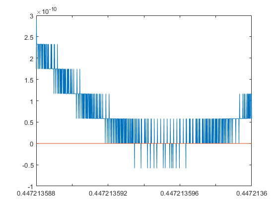
From the plot it is not clear whether there are two roots, one double root or no real root. With the pair arithmetic we can zoom much further into the critical range:
x = linspace(0.4472135954995,0.4472135955002,1000);
plot(x,double(polyval(p,cpair(x))),x,0*x)
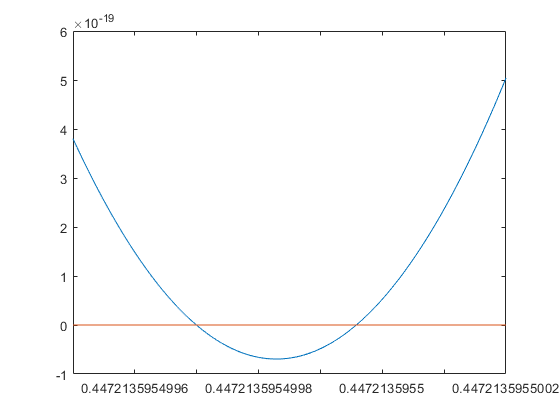
Using the pair arithmetic the polynomial values near the roots are calculated accurately. Thus, the roots may be found by a Newton iteration:
ps = [ 13953735 -4160200 -930249]

format long
K = 12;
x = cpair(0.44721);
for i=1:K
  x = x - polyval(p,x)/polyval(ps,x);
end
x1 = x

x = cpair(0.44722);
for i=1:K
  x = x - polyval(p,x)/polyval(ps,x);
end
x2 = x
ps =
    13953735    -4160200     -930249
cpair-type x1 =
   0.447213594599860
cpair-type x2 =
   0.447213597164461
Since there is an almost-double root, the convergence is slow: The approximations x1 and x2 coincide in 12 decimal figures.
From the function values at x1, x2 and at the midpoint, existence of the two roots is shown - at least numerically:
xm = ( x1 + x2 ) / 2
y1 = polyval(p,x1)
ym = polyval(p,xm)
y2 = polyval(p,x2)
cpair-type xm =
   0.447213595882160
cpair-type y1 =
     1.917295715581748e-12
cpair-type ym =
    -3.153585304293774e-12
cpair-type y2 =
     4.377955128760722e-12
Polynomial evaluation II
Now consider the following polynomial:
p = [ 194481 -629748 993178 -782664 233290 ]
p =
      194481     -629748      993178     -782664      233290
We may ask again whether this polynomial has positive roots. The following plot uses standard floating-point double precision:
m = 0.80962343;
e = 4e-8;
x = linspace(m-e,m+e,1000);
close
plot(x,polyval(p,x),x,0*x)
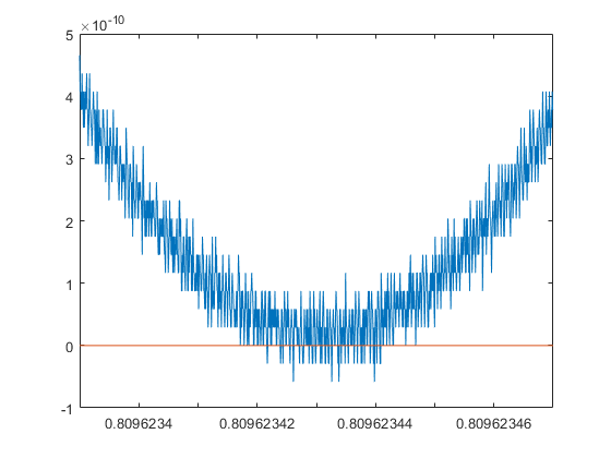
From the plot again it is not clear whether there are two roots, a double one or no one. With the pair arithmetic we calculate the minimum value over the critical range:
y = double(polyval(p,cpair(x)));
close
plot(x,y,x,0*x)

min_y = min(y)
min_y =
     1.915563615682340e-11
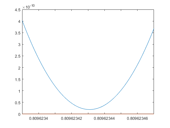
Now there is numerical evidence that in this case the polynomial has no real root near m. The minimum value of 2e-11 is too small to be calculated accurately in double precision. Thus the previous picture showed nothing but cancellation errors.
Polynomial evaluation III
As has been said, also pair-arithmetic has its limits. Once the condition number exceeds about 1e30 or so, we cannot expect correct answers. The following polynomial was constructed by Paul Zimmermann.
p = [2280476932 84854892153 114714036446 39504798003]
p =
   1.0e+11 *
  Columns 1 through 3
   0.022804769320000   0.848548921530000   1.147140364460000
  Column 4
   0.395047980030000
Again the question is whether there are real roots near -0.6954. The following graph is produced using double-double arithmetic; the graph is the same for cpair.
xs = -0.6954389494128404;
e = 3e-16;
E = linspace(-e,e,1000);
y = double(polyval(p,dd(xs)+E));
close
plot(E,y,E,0*E)
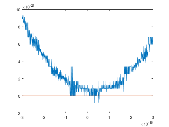
Computing in even higher precision reveals that there is no real root near xs. Note that the minimum function value is about 5e-22.
Least squares interpolation
For the previous plot we may calculate a quadratic interpolation polynomial:
p = [2280476932 84854892153 114714036446 39504798003]
xs = -0.6954389494128404;
e = 3e-16;
E = linspace(-e,e,1000)';
y = double(polyval(p,dd(xs)+E));

A = [E.^2 E ones(size(E))];
quadpoly = double(A)\y
p =
   1.0e+11 *
  Columns 1 through 3
   0.022804769320000   0.848548921530000   1.147140364460000
  Column 4
   0.395047980030000
Warning: Rank deficient, rank = 1, tol =  7.021667e-12.
quadpoly =
   1.0e-20 *
                   0
                   0
   0.295600932829705
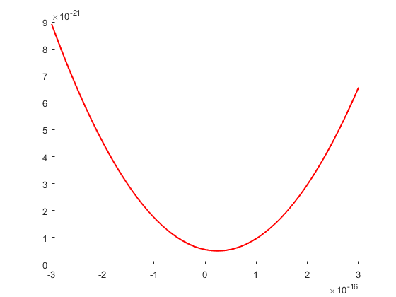
However, due to the ill-conditioning of the problem the result is just a constant. Using pair-arithmetic we may compute the true interpolation polynomial and display it.
format long e
[Q,R] = house_qr(A);
b = Q'*y;
QuadPoly = backward(R(1:3,:),b(1:3))

close, hold on
plot(E,double(polyval(QuadPoly,E)),'r','LineWidth',1.5)
hold off
QuadPoly =
     7.990425382303981e+10
    -3.927001334297470e-06
     5.540826593221900e-22
Plotting a polynomial near its roots: The Wilkinson polynomial
The values of polynomial evaluation near a root may be severely affected by rounding errors. We first evaluate the Wilkinson polynomial near its root r = 20 in cpair arithmetic:
P = poly(cpair(1:20))
e = 1e-5;
x = linspace(20-e,20+e,1000);
close
plot(x,double(polyval(P,x)))
cpair-type P =
  Columns 1 through 3
     1.000000000000000e+00    -2.100000000000000e+02     2.061500000000000e+04
  Columns 4 through 6
    -1.256850000000000e+06     5.332794600000000e+07    -1.672280820000000e+09
  Columns 7 through 9
     4.017177163000000e+10    -7.561111845000000e+11     1.131027699538100e+13
  Columns 10 through 12
    -1.355851828995300e+14     1.307535010540395e+15    -1.014229986551145e+16
  Columns 13 through 15
     6.303081209929490e+16    -3.113336431613907e+17     1.206647803780373e+18
  Columns 16 through 18
    -3.599979517947607e+18     8.037811822645051e+18    -1.287093124515099e+19
  Columns 19 through 21
     1.380375975364070e+19    -8.752948036761600e+18     2.432902008176640e+18
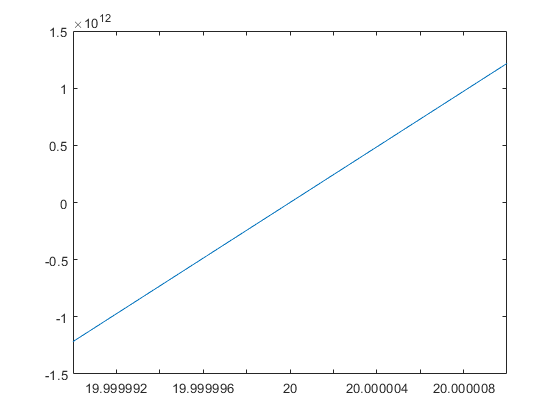
Since r = 20 is a simple root, that looks as expected. However, when evaluating in double precision the picture changes significantly:
p = poly(1:20)
close
plot(x,polyval(p,x))
p =
  Columns 1 through 3
     1.000000000000000e+00    -2.100000000000000e+02     2.061500000000000e+04
  Columns 4 through 6
    -1.256850000000000e+06     5.332794600000000e+07    -1.672280820000000e+09
  Columns 7 through 9
     4.017177163000000e+10    -7.561111845000000e+11     1.131027699538100e+13
  Columns 10 through 12
    -1.355851828995300e+14     1.307535010540395e+15    -1.014229986551145e+16
  Columns 13 through 15
     6.303081209929490e+16    -3.113336431613907e+17     1.206647803780373e+18
  Columns 16 through 18
    -3.599979517947607e+18     8.037811822645052e+18    -1.287093124515099e+19
  Columns 19 through 21
     1.380375975364070e+19    -8.752948036761600e+18     2.432902008176640e+18
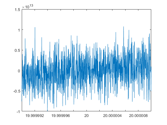
Note that all values of the polynomial are strictly positive when evaluated in double precision.
Two-term recurrences, Muller's famous example
In 1989 Jean-Michel Muller gave the following famous example of a two-term recurrence
x = [ 4 4.25 ];
for k=3:30
  x(k) = 108 - ( 815 - 1500/x(k-2) ) / x(k-1);
end
x
x =
  Columns 1 through 3
     4.000000000000000e+00     4.250000000000000e+00     4.470588235294116e+00
  Columns 4 through 6
     4.644736842105218e+00     4.770538243625083e+00     4.855700712568563e+00
  Columns 7 through 9
     4.910847498660630e+00     4.945537395530508e+00     4.966962408040999e+00
  Columns 10 through 12
     4.980042204293014e+00     4.987909232795786e+00     4.991362641314552e+00
  Columns 13 through 15
     4.967455095552268e+00     4.429690498308830e+00    -7.817236578459315e+00
  Columns 16 through 18
     1.689391676710646e+02     1.020399631520593e+02     1.000999475162497e+02
  Columns 19 through 21
     1.000049920409724e+02     1.000002495792373e+02     1.000000124786202e+02
  Columns 22 through 24
     1.000000006239216e+02     1.000000000311958e+02     1.000000000015598e+02
  Columns 25 through 27
     1.000000000000780e+02     1.000000000000039e+02     1.000000000000002e+02
  Columns 28 through 30
     1.000000000000000e+02     1.000000000000000e+02     1.000000000000000e+02
The recurrence has an attractive fixed point A = 100, and repellent fixed points R1 = 5 and R2 = 3. The initial values x0 = 4 and x1 = 4.25 are such that the recurrence converges to the repellent fixed point R1 = 5, but due to inevitable rounding errors the recurrence switches after a while to the attracting fixed point A = 100. Indeed
diff = x(29:30) - 100
diff =
     0     0
the recurrence becomes stationary at A = 100. When executing in double-double
x = dd([ 4 4.25 ]);
for k=3:280
  x(k) = 108 - ( 815 - 1500/x(k-2) ) / x(k-1);
end
iter_dd_1_40 = x(1:40)
dd-type iter_dd_1_40 =
  Columns 1 through 3
     4.000000000000000e+00     4.250000000000000e+00     4.470588235294118e+00
  Columns 4 through 6
     4.644736842105263e+00     4.770538243626063e+00     4.855700712589074e+00
  Columns 7 through 9
     4.910847499082793e+00     4.945537404123916e+00     4.966962581762701e+00
  Columns 10 through 12
     4.980045701355631e+00     4.987979448478392e+00     4.992770288062068e+00
  Columns 13 through 15
     4.995655891506634e+00     4.997391268381344e+00     4.998433943944817e+00
  Columns 16 through 18
     4.999060071970889e+00     4.999435937146743e+00     4.999661524101830e+00
  Columns 19 through 21
     4.999796900674664e+00     4.999878134702810e+00     4.999926864001790e+00
  Columns 22 through 24
     4.999955817000531e+00     4.999967474739530e+00     4.999860179403582e+00
  Columns 25 through 27
     4.997509931745810e+00     4.950357765531113e+00     3.997310528290825e+00
  Columns 28 through 30
    -2.008401887731078e+01     1.298954032591806e+02     1.011507487952248e+02
  Columns 31 through 33
     1.000568828523644e+02     1.000028425254519e+02     1.000001421222250e+02
  Columns 34 through 36
     1.000000071061009e+02     1.000000003553050e+02     1.000000000177652e+02
  Columns 37 through 39
     1.000000000008883e+02     1.000000000000444e+02     1.000000000000022e+02
  Column 40
     1.000000000000001e+02
we see the same behaviour, it only takes more iterations to reach the attractive fixed point A = 100:
diff_dd = x(278:280) - 100
dd-type diff_dd =
    2.470328229206233e-323                         0                         0
The cpair arithmetic
x = cpair([ 4 4.25 ]);
for k=3:280
  x(k) = 108 - ( 815 - 1500/x(k-2) ) / x(k-1);
end
iter_cpair_1_40 = x(1:40)
diff_cpair = x(277:280) - 100
cpair-type iter_cpair_1_40 =
  Columns 1 through 3
     4.000000000000000e+00     4.250000000000000e+00     4.470588235294118e+00
  Columns 4 through 6
     4.644736842105263e+00     4.770538243626063e+00     4.855700712589074e+00
  Columns 7 through 9
     4.910847499082793e+00     4.945537404123916e+00     4.966962581762701e+00
  Columns 10 through 12
     4.980045701355631e+00     4.987979448478392e+00     4.992770288062068e+00
  Columns 13 through 15
     4.995655891506634e+00     4.997391268381344e+00     4.998433943944821e+00
  Columns 16 through 18
     4.999060071971002e+00     4.999435937149002e+00     4.999661524147029e+00
  Columns 19 through 21
     4.999796901578719e+00     4.999878152784646e+00     4.999927225647127e+00
  Columns 22 through 24
     4.999963050010322e+00     5.000112135986626e+00     5.002753342727615e+00
  Columns 25 through 27
     5.055342782997613e+00     6.094920214787493e+00     2.296456111144083e+01
  Columns 28 through 30
     8.322733344546177e+01     9.899235870903456e+01     9.994910511016300e+01
  Columns 31 through 33
     9.999745396008689e+01     9.999987269477460e+01     9.999999363473097e+01
  Columns 34 through 36
     9.999999968173654e+01     9.999999998408683e+01     9.999999999920435e+01
  Columns 37 through 39
     9.999999999996022e+01     9.999999999999801e+01     9.999999999999990e+01
  Column 40
     1.000000000000000e+02
cpair-type diff_cpair =
  Columns 1 through 3
   -2.470328229206233e-323                         0                         0
  Column 4
                         0
produces a similar result.
Two-term recurrences, revisited
In
S.M. Rump. On recurrences converging to the wrong limit in finite
   precision and some new examples. Electr. Trans. on Num. Anal. (ETNA),
   52:358–369, 2020.
and
S.M. Rump. Addendum to "On recurrences converging to the wrong limit in
  finite precision and some new examples". Electr. Trans. on Num. Anal.
  (ETNA), 52:571–575, 2020.
a gap in the proofs is removed, namely, that it has to be shown that the recurrences are well defined for all iterates. For Muller's example that is true.
Moreover, several examples are given where rounding errors may be beneficial. Consider
x = [ -6 64 ];
for k=3:50
  x(k) = 82 - ( 1824 - 6048/x(k-2) ) / x(k-1);
end
x
x =
  Columns 1 through 3
    -6.000000000000000e+00     6.400000000000000e+01     3.775000000000000e+01
  Columns 4 through 6
     3.618543046357616e+01     3.602049780380673e+01     3.600227623770425e+01
  Columns 7 through 9
     3.600025289930995e+01     3.600002809972593e+01     3.600000312218934e+01
  Columns 10 through 12
     3.600000034690991e+01     3.600000003854556e+01     3.600000000428285e+01
  Columns 13 through 15
     3.600000000047589e+01     3.600000000005290e+01     3.600000000000590e+01
  Columns 16 through 18
     3.600000000000068e+01     3.600000000000011e+01     3.600000000000005e+01
  Columns 19 through 21
     3.600000000000005e+01     3.600000000000006e+01     3.600000000000006e+01
  Columns 22 through 24
     3.600000000000008e+01     3.600000000000009e+01     3.600000000000011e+01
  Columns 25 through 27
     3.600000000000012e+01     3.600000000000014e+01     3.600000000000017e+01
  Columns 28 through 30
     3.600000000000020e+01     3.600000000000023e+01     3.600000000000026e+01
  Columns 31 through 33
     3.600000000000031e+01     3.600000000000036e+01     3.600000000000042e+01
  Columns 34 through 36
     3.600000000000049e+01     3.600000000000057e+01     3.600000000000066e+01
  Columns 37 through 39
     3.600000000000077e+01     3.600000000000090e+01     3.600000000000104e+01
  Columns 40 through 42
     3.600000000000122e+01     3.600000000000143e+01     3.600000000000167e+01
  Columns 43 through 45
     3.600000000000195e+01     3.600000000000227e+01     3.600000000000265e+01
  Columns 46 through 48
     3.600000000000309e+01     3.600000000000361e+01     3.600000000000421e+01
  Columns 49 through 50
     3.600000000000492e+01     3.600000000000574e+01
with attractive fixed point A = 42 and repellent fixed points R1 = 36 and R2 = 4. At first sight it looks as if the double precision iteration converges to the repellent fixed point R1 = 36. However, continuing with the iteration reveals that after some 450 iterates the recurrence becomes stationary at the attractive fixed point A = 42:
x = [ -6 64 ];
for k=3:450
  x(k) = 82 - ( 1824 - 6048/x(k-2) ) / x(k-1);
end
diff_double = x(445:450) - 42
diff_double(1) == diff_double
diff_double =
  Columns 1 through 3
    -2.842170943040401e-14    -2.842170943040401e-14    -2.842170943040401e-14
  Columns 4 through 6
    -2.842170943040401e-14    -2.842170943040401e-14    -2.842170943040401e-14
ans =
  1×6 logical array
   1   1   1   1   1   1
The result in double-double is
x = dd([ -6 64 ]);
for k=3:5300
  x(k) = 82 - ( 1824 - 6048/x(k-2) ) / x(k-1);
end
x_dd_end = x(end-5:end)
close
plot(double(x))
x(end-5:end) == 42
dd-type x_dd_end =
    42    42    42    42    42    42
ans =
  1×6 logical array
   1   1   1   1   1   1

also converging to the attractive fixed point A = 42. However, cpair arithmetic yields:
x = cpair([ -6 64 ]);
for k=3:20
  x(k) = 82 - ( 1824 - 6048/x(k-2) ) / x(k-1);
end
x
close
plot(double(x))
x == 36
cpair-type x =
  Columns 1 through 3
    -6.000000000000000e+00     6.400000000000000e+01     3.775000000000000e+01
  Columns 4 through 6
     3.618543046357616e+01     3.602049780380673e+01     3.600227623770425e+01
  Columns 7 through 9
     3.600025289930995e+01     3.600002809972592e+01     3.600000312218933e+01
  Columns 10 through 12
     3.600000034690989e+01     3.600000003854554e+01     3.600000000428284e+01
  Columns 13 through 15
     3.600000000047587e+01     3.600000000005287e+01     3.600000000000588e+01
  Columns 16 through 18
     3.600000000000065e+01     3.600000000000007e+01     3.600000000000001e+01
  Columns 19 through 20
     3.600000000000000e+01     3.600000000000000e+01
ans =
  1×20 logical array
  Columns 1 through 19
   0   0   0   0   0   0   0   0   0   0   0   0   0   0   0   0   0   0   1
  Column 20
   1

So for cpair arithmetic, due to beneficial rounding errors, the recurrence converges to the repellent fixed point R1 = 36. Luckily, that is the correct result when computing in infinite precision.
Enjoy INTLAB
INTLAB was designed and written by S.M. Rump, head of the Institute for Reliable Computing, Hamburg University of Technology. Suggestions are always welcome to rump (at) tuhh.de