DEMOINTLAB_FACTORIZATIONS Verified bounds for matrix factors

From INTLAB Version 14 algorithms are included to compute verified bounds for the factors of many standard matrix factorizations. The inclusions are subject to uniqueness, i.e., for ill-posed problems the factors are not unique and verified bounds cannot be computed because the problem becomes ill-posed.

Matrix factorizations
The LU-factorization
Limits to verified bounds for the LU-factorization
The singular value decomposition
The eigenvalue decomposition
Rank verification
Factorizations of interval matrices
The QR-decomposition
The Cholesky decomposition
Cholesky factors of larger matrices
The Schur decomposition
The polar and Takagi decomposition
Enjoy INTLAB

Matrix factorizations

A trivial example is the svd-decomposition of the identity matrix where U I U^T is a valid factorization for any unitary U.

Most of the factorization algorithms are based on

  S.M. Rump and T. Ogita. Verified error bounds for matrix decompositions.
    SIAM Journal on Matrix Analysis and Applications (SIMAX), 45(4),
    2155–2183, 2024.

The methods are based on so-called perturbations of 1, i.e., the problem is transformed into a matrix close to the identity matrix. That method turned out to be fruitful in many applications and is used in other algorithms in INTLAB.

The syntax for INTLAB's verification algorithms to calculate verified inclusions of factors of a matrix are close to or identical to the Matlab notation. The only difference is that the input matrix is of type intval.

To avoid the type cast all routines are offered in two versions. For example, the calls

  [Q,R] = qr(intval(A))   and   [Q,R] = verifyqr(A)

are identical for a (real or complex) point matrix A.

The LU-factorization

Consider the 4x4 scaled Hilbert matrix

setround(0)
format short _
n = 4;
A = hilbert(n)

A =
   420   210   140   105
   210   140   105    84
   140   105    84    70
   105    84    70    60

with the scaling of the original Hilbert matrix hilb(n) to integer entries, that is the entries multiplied by the least common multiple of 1...2n-1. For n=4 the factor is 420, appearing in the left upper corner of hilbert(n). An approximate lu-decomposition is computed by

[L,U] = lu(A)

L =
    1.0000         0         0         0
    0.5000    1.0000         0         0
    0.3333    1.0000    0.6667    1.0000
    0.2500    0.9000    1.0000         0
U =
  420.0000  210.0000  140.0000  105.0000
         0   35.0000   35.0000   31.5000
         0         0    3.5000    5.4000
         0         0         0   -0.1000

Note that theoretically no pivoting is necessary because the matrix is symmetric positive definite, but numerically some pivoting occurs.

The dimension is small and the matrix well-conditioned. Therefore it is no big problem to compute inclusions of the factors. To see the accuracy of the inclusions we change the format to long:

format long _
[Lint,Uint] = lu(intval(A))
format short _

intval Lint = 
   1.00000000000000   0.00000000000000   0.00000000000000   0.00000000000000
   0.50000000000000   1.00000000000000   0.00000000000000   0.00000000000000
   0.33333333333333   1.00000000000000   0.66666666666666   1.00000000000000
   0.25000000000000   0.90000000000000   1.00000000000000   0.00000000000000
intval Uint = 
  1.0e+002 *
   4.20000000000000   2.10000000000000   1.40000000000000   1.05000000000000
   0.00000000000000   0.35000000000000   0.35000000000000   0.31500000000000
   0.00000000000000   0.00000000000000   0.03500000000000   0.05400000000000
   0.00000000000000   0.00000000000000   0.00000000000000  -0.00100000000000

As no underscore is seen, all displayed figures are correct (see help intvalinit). A quick check

in(A,Lint*Uint)

ans =
  4×4 logical array
   1   1   1   1
   1   1   1   1
   1   1   1   1
   1   1   1   1

is no proof of correctness; necessarily the result must be a matrix of 1's.

The type cast intval(.) is necessary to tell INTLAB that an inclusion of the factors rather than an approximation is wanted. An alternative call without type cast is

[Lint,Uint] = verifylu(A);

The accuracy of Matlab's approximation can be monitored by changing to a larger dimension. We choose n=11, and as before numerical instabilities cause some pivoting. In order to ensure that the L-factor is lower triangular we add the explicit pivot information P as a third output parameter:

n = 11;
A = hilbert(n);
condA = cond(A)
[L,U,P] = lu(A,'vector');
[Lint,Uint,p] = lu(intval(A),'vector');

condA =
   5.2283e+14

A quick check as before is

in( A(p,:) , Lint*Uint )

ans =
  11×11 logical array
   1   1   1   1   1   1   1   1   1   1   1
   1   1   1   1   1   1   1   1   1   1   1
   1   1   1   1   1   1   1   1   1   1   1
   1   1   1   1   1   1   1   1   1   1   1
   1   1   1   1   1   1   1   1   1   1   1
   1   1   1   1   1   1   1   1   1   1   1
   1   1   1   1   1   1   1   1   1   1   1
   1   1   1   1   1   1   1   1   1   1   1
   1   1   1   1   1   1   1   1   1   1   1
   1   1   1   1   1   1   1   1   1   1   1
   1   1   1   1   1   1   1   1   1   1   1

The matrix is already pretty ill-conditioned with condition number 5e14. In order to compute the median and maximum relative error of the inclusion and of the approximation we have to exclude the lower and upper triangular part because by definition these are all zero.

index = find(triu(ones(n)));
relerrLint = relerr(Lint);
relerrLint(index) = [];
relerrL = relerr(L,Lint);
relerrL(index) = [];
format shorte
relerrL = [median(relerrLint(:)) max(relerrLint(:)) median(relerrL(:)) max(relerrL(:))]

relerrL =
   9.6470e-16   5.5765e-11   9.9920e-16   4.7512e-07

The first two numbers show the median and maximum relative error of the inclusion of the L-factor, and the third and fourth number the accuracy of the approximation of L by Matlab's lu. As can be seen in the median the inclusions are maximally accurate, where at least 11 digits of the inclusion are guaranteed. In the median Matlab's approximation is maximally accurate as well, but in the worst case some 7 digits are correct.

The same information for the U-factor is as follows:

index = find(tril(ones(n),-1));
relerrUint = relerr(Uint);
relerrUint(index) = [];
relerrU = relerr(U,Uint);
relerrU(index) = [];
relerrU = [median(relerrUint(:)) max(relerrUint(:)) median(relerrU(:)) max(relerrU(:))]

relerrU =
   2.5404e-16   5.2105e-08   3.4809e-16   1.7413e-04

Now the inclusion of the U-factor is correct to at least 8 figures, in the median it is maximally accurate as for the L-factor. The approximation of the U-factor has entries with 4 correct digits. That result is computed by Matlab's backslash without warning.

Limits to verified bounds for the LU-factorization

If the matrix is too ill-conditioned, the results are NaNs, indicating that the verification failed. For the Hilbert matrix the limit is n = 12:

n = 12;
A = hilbert(n);
[Lint,Uint,p] = lu(intval(A),'vector');
Uint(1)

intval ans = 
          NaN

Even for a singular matrix it is no problem to compute approximate LU-factors by Matlab's backslash. Usually a warning is given if the matrix condition number is close to 1/u ~ 1e16.

For n = 12 we use the Advanpix multiple precision package to judge the accuracy of Matlab's backslash. Although this information is not verified to be correct it is very likely correct because the mp-package uses extended precision:

[L,U,P] = lu(A,'vector');
mp.Digits(34);
[Lmp,Ump,Pmp] = lu(mp(A),'vector');
relUend = relerr(U(end),double(Ump(end)))
relerrU = relerr(U,double(Ump));
maxrelerrU = max(relerrU(:))

relUend =
   4.1895e-03
maxrelerrU =
   4.1895e-03

As can be seen some entries of Matlab's U-factor have only 3 correct digits without warning. For more details refer to

  help intval/lu   or   help verifylu

The singular value decomposition

The call of verifysvd or svd(intval(.)) is adapted from Matlab's singular value decomposition. The verification routines are based on

S.M. Rump and M. Lange. Fast computation of error bounds for all
  eigenpairs of a Hermitian and all singular pairs of a rectangular matrix
  with emphasis on eigen- and singular value clusters. Journal of
  Computational and Applied Mathematics (JCAM), 434:115332, 2023.

For example

format short _
m = 5; n = 3; A = randn(m,n);
[U,S,V] = svd(intval(A))

intval U = 
   -0.8219    0.0175   -0.4410    0.1384    0.3322
    0.0392    0.1190   -0.4769   -0.8492   -0.1885
    0.4741   -0.0462   -0.7581    0.4449   -0.0164
   -0.0548    0.9535    0.0155    0.1752   -0.2383
    0.3083    0.2723    0.0535   -0.1759    0.8927
intval S = 
    2.7472    0.0000    0.0000
    0.0000    1.8824    0.0000
    0.0000    0.0000    0.5684
    0.0000    0.0000    0.0000
    0.0000    0.0000    0.0000
intval V = 
   -0.7129   -0.6333    0.3010
    0.5832   -0.7739   -0.2467
    0.3893   -0.0003    0.9211

By default the full singular value decomposition is computed. As for Matlab's svd an inclusion of the economy size decomposition is obtained as well:

[U,S,V] = verifysvd(A,'econ')

intval U = 
   -0.8219    0.0175   -0.4410
    0.0392    0.1190   -0.4769
    0.4741   -0.0462   -0.7581
   -0.0548    0.9535    0.0155
    0.3083    0.2723    0.0535
intval S = 
    2.7472    0.0000    0.0000
    0.0000    1.8824    0.0000
    0.0000    0.0000    0.5684
intval V = 
   -0.7129   -0.6333    0.3010
    0.5832   -0.7739   -0.2467
    0.3893   -0.0003    0.9211

in which case the matrix S of singular values is diagonal. The relative error of the inclusions is as follows:

relU = relerr(U);
relS = relerr(diag(S));
relV = relerr(V);
medianrelUSV = [median(relU(:)) median(relS) median(relV(:))]
maxrelUSV = [max(relU(:)) max(relS) max(relV(:))]

medianrelUSV =
   1.0e-13 *
    0.1494    0.0089    0.0585
maxrelUSV =
   1.0e-11 *
    0.0236    0.0001    0.8838

So in the median some 14 and at least 13 digits are gueranteed. Next

resUSV = all(all(in( A , U*S*V' )))
resU = all(all( in( 0 , U'*U - eye(n) )))
resV = all(all( in( 0 , V'*V - eye(n) )))

resUSV =
  logical
   1
resU =
  logical
   1
resV =
  logical
   1

does neither prove that U and V are inclusions of the factors nor that U and V are orthogonal, but values true are a necessary condition. For more details refer to

  help intval/svd   or   help verifysvd

The eigenvalue decomposition

Again the call is similar to Matlab's eig:

n = 5;
A = reshape(1:n^2,n,n)
L = eig(intval(A))

A =
     1     6    11    16    21
     2     7    12    17    22
     3     8    13    18    23
     4     9    14    19    24
     5    10    15    20    25
intval L = 
  68.6420 -  0.0000i 
  -3.6420 +  0.0000i 
   0.0000 -  0.0000i 
   0.0000 -  0.0000i 
   0.0000 -  0.0000i

The inclusion L of the eigenvalues indicate that there are three zero eigenvalues corresponding to rank(A)=2. Indeed

r = rank(A)
R = rank(intval(A))

r =
     2
intval R = 
[    2.0000,    5.0000]

proves that the rank is at least 2. Note that an epsilon-perturbation of A may change the matrix to full rank, therefore - if not computing symbolically without rounding error - a verified upper bound for the rank must be 5. An inclusion of eigenvectors with an indication of correctness is obtained by

[X,L] = eig(intval(A))
in( A , (X*L)/X )

intval X = 
  -0.3800 -  0.0000i   -0.7670 +  0.0000i    0.1903 +  0.0000i   -0.0024 -  0.0043i   -0.0024 +  0.0043i 
  -0.4124 -  0.0000i   -0.4859 +  0.0000i   -0.4559 +  0.0000i   -0.0646 +  0.0846i   -0.0646 -  0.0846i 
  -0.4448 -  0.0000i   -0.2047 +  0.0000i   -0.0762 +  0.0000i   -0.3099 -  0.1182i   -0.3099 +  0.1182i 
  -0.4772 +  0.0000i    0.0763 -  0.0000i    0.7589 -  0.0000i    0.8233 -  0.0000i    0.8233 +  0.0000i 
  -0.5096 -  0.0000i    0.3574 +  0.0000i   -0.4171 -  0.0000i   -0.4463 +  0.0379i   -0.4463 -  0.0379i 
intval L = 
  68.6420 -  0.0000i    0.0000 +  0.0000i    0.0000 +  0.0000i    0.0000 +  0.0000i    0.0000 +  0.0000i 
   0.0000 +  0.0000i   -3.6420 +  0.0000i    0.0000 +  0.0000i    0.0000 +  0.0000i    0.0000 +  0.0000i 
   0.0000 +  0.0000i    0.0000 +  0.0000i    0.0000 -  0.0000i    0.0000 +  0.0000i    0.0000 +  0.0000i 
   0.0000 +  0.0000i    0.0000 +  0.0000i    0.0000 +  0.0000i    0.0000 -  0.0000i    0.0000 +  0.0000i 
   0.0000 +  0.0000i    0.0000 +  0.0000i    0.0000 +  0.0000i    0.0000 +  0.0000i    0.0000 -  0.0000i 
ans =
  5×5 logical array
   1   1   1   1   1
   1   1   1   1   1
   1   1   1   1   1
   1   1   1   1   1
   1   1   1   1   1

Rank verification

Another way to check for the rank is to compute an interval matrix Delta with the property that Delta contains a matrix E such that A-E is singular:

Delta = verifyrankpert(A)
in( 0 , Delta )

intval Delta = 
  1.0e-014 *
   -0.0___   -0.0___    0.____   -0.0___   -0.0___
    0.0___    0.0___   -0.____    0.0___    0.0___
   -0.0___   -0.0___    0.____   -0.0___   -0.0___
   -0.0___   -0.0___    0.____   -0.0___   -0.0___
    0.0___    0.0___   -0.____    0.0___    0.0___
ans =
  5×5 logical array
   1   1   1   1   1
   1   1   1   1   1
   1   1   1   1   1
   1   1   1   1   1
   1   1   1   1   1

We anticipate that the matrix A is singular, therefore a zero perturbation is a singular matrix. The method verifyrankpert is based on

M. Lange and S.M. Rump. Verified inclusions of a nearest matrix of
  specified rank deficiency via a generalization of Wedin's sin (θ)
  theorem [winner of the Moore prize 2021].
  BIT Numerical Mathematics, 61:361–380, 2021.

Note that we used verifyeigall, in contrast to lu and svd where verifylu and verifysvd is used. The reason is that from the beginning of INTLAB the routine verifyeig is reserved to compute inclusions of one (single or multiple) eigenvalue together with inclusions of an invariant subspace, see the demo dintval (Some examples of interval computations).

Methods for symmetric/Hermitian matrices are based on

S.M. Rump and M. Lange. Fast computation of error bounds for all
  eigenpairs of a Hermitian and all singular pairs of a rectangular matrix
  with emphasis on eigen- and singular value clusters. Journal of
  Computational and Applied Mathematics (JCAM), 434:115332, 2023.

and for general matrices based on

S.M. Rump. Verified error bounds for all eigenvalues and eigenvectors of a matrix.
   SIAM Journal Matrix Analysis (SIMAX), 43:1736-1754, 2022.

For more details refer to

  help intval/eig   or   help verifyeigall

Factorizations of interval matrices

Consider the 4x4 scaled Hilbert matrix which we now afflict with an entrywise absolute error 1e-10:

n = 4;
Aint = midrad(hilbert(n),1e-10)

intval Aint = 
  420.0000  210.0000  140.0000  105.0000
  210.0000  140.0000  105.0000   84.0000
  140.0000  105.0000   84.0000   70.0000
  105.0000   84.0000   70.0000   60.0000

To see the intervals we change the format to long:

format long _
Aint

intval Aint = 
  1.0e+002 *
   4.200000000000__   2.100000000000__   1.400000000000__   1.050000000000__
   2.100000000000__   1.400000000000__   1.050000000000__   0.840000000000__
   1.400000000000__   1.050000000000__   0.840000000000__   0.700000000000__
   1.050000000000__   0.840000000000__   0.700000000000__   0.600000000000__

When computing a factorization of the interval matrix Aint, the factors of all matrices A in Aint are included. Of course, this widens the inclusions:

[Lint,Uint] = lu(Aint)

intval Lint = 
   1.00000000000000   0.00000000000000   0.00000000000000   0.00000000000000
   0.500000000000__   1.00000000000000   0.00000000000000   0.00000000000000
   0.333333333333__   1.0000000000____   0.666666667_____   1.00000000000000
   0.250000000000__   0.9000000000____   1.00000000000000   0.00000000000000
intval Uint = 
  1.0e+002 *
   4.20000000000___   2.10000000000___   1.40000000000___   1.05000000000___
   0.00000000000000   0.35000000000___   0.35000000000___   0.3150000000____
   0.00000000000000   0.00000000000000   0.03500000000___   0.0540000000____
   0.00000000000000   0.00000000000000   0.00000000000000  -0.00100000000___

If the input intervals are too wide, singular matrices move into it and an inclusion is not possible:

format short _
for e=[0.001 0.01 0.1]
  e
  [Lint,Uint] = lu(midrad(hilbert(n),e))
end

e =
   1.0000e-03
intval Lint = 
    1.0000    0.0000    0.0000    0.0000
    0.5000    1.0000    0.0000    0.0000
    0.3333    1.000_    0.67__    1.0000
    0.2500    0.900_    1.0000    0.0000
intval Uint = 
  420.00__  210.00__  140.00__  105.00__
    0.0000   35.00__   35.00__   31.5___
    0.0000    0.0000    3.50__    5.4___
    0.0000    0.0000    0.0000   -0.10__
e =
    0.0100
intval Lint = 
    1.0000    0.0000    0.0000    0.0000
    0.5000    1.0000    0.0000    0.0000
    0.3333    1.00__    0.7___    1.0000
    0.2500    0.90__    1.0000    0.0000
intval Uint = 
[  419.9899,  420.0101] [  209.9799,  210.0201] [  139.9599,  140.0401] [  104.9181,  105.0819] 
[    0.0000,    0.0000] [   34.9774,   35.0226] [   34.9449,   35.0551] [   31.3809,   31.6191] 
[    0.0000,    0.0000] [    0.0000,    0.0000] [    3.4544,    3.5456] [    5.2615,    5.5385] 
[    0.0000,    0.0000] [    0.0000,    0.0000] [    0.0000,    0.0000] [   -0.1692,   -0.0308] 
e =
    0.1000
intval Lint = 
       NaN       NaN       NaN       NaN
       NaN       NaN       NaN       NaN
       NaN       NaN       NaN       NaN
       NaN       NaN       NaN       NaN
intval Uint = 
       NaN       NaN       NaN       NaN
       NaN       NaN       NaN       NaN
       NaN       NaN       NaN       NaN
       NaN       NaN       NaN       NaN

For e = 0.01 the intervals are wide, but still correct. That means, the LU-factors of any entrywise absolute perturbation of hilbert(4) less than or equal to 0.01 are members of the computed inclusions.

For e = 0.1 no inclusions are possible, presumably because the interval matrix contains a singular matrix. This can be verified:

A = midrad(hilbert(n),0.1)
Eint = verifyrankpert(A.mid)

intval A = 
  420.0___  210.0___  140.0___  105.0___
  210.0___  140.0___  105.0___   84.0___
  140.0___  105.0___   84.0___   70.0___
  105.0___   84.0___   70.0___   60.0___
intval Eint = 
    0.0001   -0.0003    0.0009   -0.0006
   -0.0003    0.0043   -0.0105    0.0068
    0.0009   -0.0105    0.0254   -0.0165
   -0.0006    0.0068   -0.0165    0.0107

As has been described before, the interval matrix Eint contains a matrix E such that A.mid-E is singular. Now all entries of Eint are less than 0.1 in absolute value

abs(Eint) <= 0.1

ans =
  4×4 logical array
   1   1   1   1
   1   1   1   1
   1   1   1   1
   1   1   1   1

so that indeed the input matrix Aint = midrad(hilbert(n),0.1) contains a singular matrix.

Other factorizations of interval matrices are possible, for exmaple

[U,S,V] = svd(midrad(hilbert(4),1e-4))

intval U = 
   -0.7926    0.5821   -0.179_   -0.029_
   -0.4519   -0.3705    0.742_    0.329_
   -0.3224   -0.5096   -0.100_   -0.791_
   -0.2521   -0.5140   -0.638_    0.515_
intval S = 
  630.090_    0.0000    0.0000    0.0000
    0.0000   71.039_    0.0000    0.0000
    0.0000    0.0000    2.830_    0.0000
    0.0000    0.0000    0.0000    0.041_
intval V = 
   -0.7926    0.5821   -0.179_   -0.029_
   -0.4519   -0.3705    0.742_    0.329_
   -0.3224   -0.5096   -0.100_   -0.791_
   -0.2521   -0.5140   -0.638_    0.515_

This applies to complex interval matrices as well:

A = hilbert(4) + 1i*pascal(4)
[U,S,V] = svd(midrad(A,1e-4))

A =
   1.0e+02 *
   4.2000 + 0.0100i   2.1000 + 0.0100i   1.4000 + 0.0100i   1.0500 + 0.0100i
   2.1000 + 0.0100i   1.4000 + 0.0200i   1.0500 + 0.0300i   0.8400 + 0.0400i
   1.4000 + 0.0100i   1.0500 + 0.0300i   0.8400 + 0.0600i   0.7000 + 0.1000i
   1.0500 + 0.0100i   0.8400 + 0.0400i   0.7000 + 0.1000i   0.6000 + 0.2000i
intval U = 
  -0.7922 +  0.0025i    0.5715 +  0.0513i   -0.183_ -  0.0657i    0.072_ +  0.010_i 
  -0.4518 -  0.0017i   -0.3504 +  0.0154i    0.5412 +  0.332_i   -0.5029 -  0.130_i 
  -0.3226 -  0.0071i   -0.4967 -  0.0574i    0.0960 +  0.108_i    0.730_ +  0.302_i 
  -0.2527 -  0.0144i   -0.5194 -  0.1670i   -0.492_ -  0.545_i   -0.2568 -  0.184_i 
intval S = 
  630.309_    0.0000    0.0000    0.0000
    0.0000   73.577_    0.0000    0.0000
    0.0000    0.0000    7.852_    0.0000
    0.0000    0.0000    0.0000    0.369_
intval V = 
  -0.7922 +  0.0000i    0.5738 +  0.0000i   -0.194_ +  0.0000i    0.073_ +  0.0000i 
  -0.4518 +  0.0031i   -0.3477 -  0.0467i    0.621_ -  0.1292i   -0.516_ +  0.057_i 
  -0.3226 +  0.0082i   -0.4999 +  0.0128i    0.127_ -  0.069_i    0.7661 -  0.195_i 
  -0.2526 +  0.0152i   -0.5322 +  0.1199i   -0.647_ +  0.346_i   -0.280_ +  0.146_i

The QR-decomposition

Consider

format short
m = 5; n = 3; A = randn(m,n);
[Q,R] = qr(intval(A))

intval Q = 
   -0.0306   -0.0230    0.7597    0.4453   -0.4722
    0.4359   -0.3228    0.4077   -0.7329   -0.0477
   -0.2751   -0.1776   -0.3859   -0.2462   -0.8265
    0.4954   -0.6913   -0.2759    0.4471   -0.0206
   -0.6984   -0.6210    0.1774   -0.0628    0.3018
intval R = 
    1.7082   -0.9173    1.3036
    0.0000   -1.7432   -1.2093
    0.0000    0.0000   -1.6716
    0.0000    0.0000    0.0000
    0.0000    0.0000    0.0000

As before the quick check

in(A,Q*R)
in( eye(m) , Q'*Q )

ans =
  5×3 logical array
   1   1   1
   1   1   1
   1   1   1
   1   1   1
   1   1   1
ans =
  5×5 logical array
   1   1   1   1   1
   1   1   1   1   1
   1   1   1   1   1
   1   1   1   1   1
   1   1   1   1   1

does not prove correctness but must necessarily produce only 1's. As for Matlab's qr-decomposition inclusions of economy size factors are possible as well:

[Q,R] = qr(intval(A),'econ')

intval Q = 
   -0.0306   -0.0230    0.7597
    0.4359   -0.3228    0.4077
   -0.2751   -0.1776   -0.3859
    0.4954   -0.6913   -0.2759
   -0.6984   -0.6210    0.1774
intval R = 
    1.7082   -0.9173    1.3036
    0.0000   -1.7432   -1.2093
    0.0000    0.0000   -1.6716

Now R is an upper triangular square matrix. For more details refer to

  help intval/qr   or   help verifyqr

The Cholesky decomposition

A symmetric positive semidefinite matrix allows a Cholesky decomposition. Consider a random s.p.d. matrix with condition number 1e12:

n = 10;
A = gallery('randsvd',n,-1e12);
condA = cond(A)
G = verifychol(A);

condA =
   9.9999e+11

The result of the verified inclusion G satisfies the quick check

in( A , G'*G )

ans =
  10×10 logical array
   1   1   1   1   1   1   1   1   1   1
   1   1   1   1   1   1   1   1   1   1
   1   1   1   1   1   1   1   1   1   1
   1   1   1   1   1   1   1   1   1   1
   1   1   1   1   1   1   1   1   1   1
   1   1   1   1   1   1   1   1   1   1
   1   1   1   1   1   1   1   1   1   1
   1   1   1   1   1   1   1   1   1   1
   1   1   1   1   1   1   1   1   1   1
   1   1   1   1   1   1   1   1   1   1

As for the previous algorithms, verifychol applies to Hermitian positive definite matrices as well:

n = 5;
A = randomc(n);
A = A'*A
G = verifychol(A)
in( A , G'*G )

A =
  Columns 1 through 4
   4.5825 + 0.0000i  -0.0385 + 0.6353i  -2.1514 - 1.0250i   0.1737 + 1.2529i
  -0.0385 - 0.6353i   3.0157 + 0.0000i  -1.6242 + 0.6049i   0.4237 - 0.4241i
  -2.1514 + 1.0250i  -1.6242 - 0.6049i   3.4674 + 0.0000i   0.1803 + 0.2974i
   0.1737 - 1.2529i   0.4237 + 0.4241i   0.1803 - 0.2974i   2.2721 + 0.0000i
   0.5630 - 0.0355i   0.3580 + 0.7631i  -0.1363 - 1.6481i   0.9280 - 1.5882i
  Column 5
   0.5630 + 0.0355i
   0.3580 - 0.7631i
  -0.1363 + 1.6481i
   0.9280 + 1.5882i
   4.1391 + 0.0000i
intval G = 
   2.1406 +  0.0000i   -0.0179 +  0.2967i   -1.0049 -  0.4788i    0.0811 +  0.5852i    0.2630 +  0.0165i 
   0.0000 +  0.0000i    1.7109 -  0.0000i   -0.8768 +  0.1741i    0.1469 -  0.2276i    0.2091 -  0.4002i 
   0.0000 +  0.0000i    0.0000 +  0.0000i    1.1954 +  0.0000i    0.5944 +  0.5628i    0.3254 +  1.0241i 
   0.0000 +  0.0000i    0.0000 +  0.0000i    0.0000 +  0.0000i    1.0860 +  0.0000i    0.0048 +  1.2213i 
   0.0000 +  0.0000i    0.0000 +  0.0000i    0.0000 +  0.0000i    0.0000 +  0.0000i    1.1041 -  0.0000i 
ans =
  5×5 logical array
   1   1   1   1   1
   1   1   1   1   1
   1   1   1   1   1
   1   1   1   1   1
   1   1   1   1   1

Following a test with a matrix close to being not definite:

n = 13;
A = hilbert(n);
Gint = chol(intval(A));
G = chol(A);
Gintend = Gint(end)
Gend = G(end)
Gmp = chol(mp(A));
double(Gmp(end))

intval Gintend = 
[    0.0114,    0.0130] 
Gend =
    0.0170
ans =
    0.0121

To save space we only look at the lower right element of the Cholesky factor. The inclusion is not accurate, guaranteeing only one digit. However, Matlab's chol produces the approximation 0.0170 which is outside the bounds. Using extended precision and the mp-toolbox gives 0.0121 as the result, basically the midpoint of the inclusion. For more details refer to

  help intval/chol   or   help verifychol

Cholesky factors of larger matrices

Following we compute an inclusion of the Cholesky factor of a complex of dimension n = 100 and plot the relative error of the inclusion:

n = 100;
A = randomc(n);
G = verifychol(A'*A);
v = 1:n;
[X,Y] = meshgrid(v,v);
rel = relerr(flipud(G));
medianmaxrel = [median(rel(:)) max(rel(:))]
Z = log(rel);
close
surface(X,Y,Z)

medianmaxrel =
   1.0e-13 *
    0.0057    0.1052

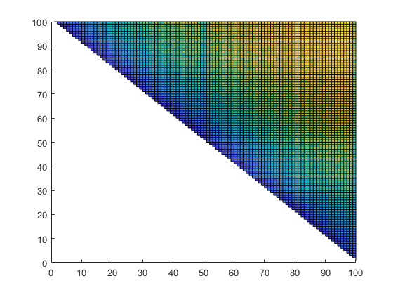
The inclusion is of almost maximal accuracy. For a complex matrix of dimension n = 1000 at least 13 correct digits are verified, in the median inclusions are maximally accurate:

n = 1000;
A = randomc(n);
G = verifychol(A'*A);
rel = relerr(flipud(G));
medianmaxrel = [median(rel(:)) max(rel(:))]

medianmaxrel =
   1.0e-13 *
    0.0056    0.7201

The Schur decomposition

Since the Schur decomposition not unique it is difficult to compare Matlab's approximation and our inclusion. However, at least the diagonal of T are the eigenvalues and should be equal:

n = 5;
A = randn(n);
[U,T] = schur(A,'complex');
[Uint,Tint] = verifyschur(A);
format long _
diagT = diag(T)
diagTint = diag(Tint)

diagT =
  1.352368119525900 + 0.000000000000000i
 -1.036879531595105 + 1.648441373372141i
 -1.036879531595105 - 1.648441373372141i
 -0.281831063707282 + 0.000000000000000i
 -0.737227859885611 + 0.000000000000000i
intval diagTint = 
   1.35236811952590 +  0.00000000000000i 
  -1.0368795315951_ +  1.64844137337214i 
  -1.0368795315951_ -  1.64844137337214i 
  -0.28183106370728 -  0.00000000000000i 
  -0.73722785988561 +  0.00000000000000i

In the long format _ no underscore is seen, thus all displayed digits of the inclusion are correct.

The Frobenius norm of the nilpotent part of T is the distance of A to normality, so that the norms of T and Tint should be equal:

normT = norm(T,'fro')
normTint = norm(Tint,'fro')
format short _

normT =
   5.443429767195253
intval normTint = 
   5.443429767195__

Note that the computation of the real Schur decomposition is an ill-posed problem and can therefore not be supported by verification routines. For more details refer to

  help intval/schur   or   help verifyschur

The polar and Takagi decomposition

Inclusions of the singular factors allow to compute inclusions of the polar and Takagi decomposition. Examples are

n = 5;
A = randn(n);
[Q,P] = verifypolar(A)
in( A , Q*P )
in( eye(n) , Q'*Q )

intval Q = 
    0.0237   -0.6084   -0.6636   -0.3089   -0.3055
   -0.1379    0.6249   -0.0890   -0.4190   -0.6379
    0.1781    0.2827   -0.5205    0.7624   -0.1897
   -0.5748    0.2890   -0.4785   -0.1560    0.5768
   -0.7862   -0.2752    0.2274    0.3510   -0.3619
intval P = 
    0.9030    0.7236    0.0417   -0.3765   -0.4409
    0.7236    3.2184   -0.2354    0.1947    0.4836
    0.0417   -0.2354    0.5129    0.2409    0.0776
   -0.3765    0.1947    0.2409    1.4531    0.0867
   -0.4409    0.4836    0.0776    0.0867    1.2475
ans =
  5×5 logical array
   1   1   1   1   1
   1   1   1   1   1
   1   1   1   1   1
   1   1   1   1   1
   1   1   1   1   1
ans =
  5×5 logical array
   1   1   1   1   1
   1   1   1   1   1
   1   1   1   1   1
   1   1   1   1   1
   1   1   1   1   1

and

n = 5;
A = randomc(n);
A = A + A.'
[U,S] = takagi(intval(A))
in( A , U*S*U.' )
in( eye(n) , U'*U )

A =
  Columns 1 through 4
   0.6215 + 1.5273i   0.9440 + 0.5689i  -0.6875 + 0.8806i  -0.2335 - 0.7700i
   0.9440 + 0.5689i   0.0691 - 1.1861i  -0.2415 + 0.5816i  -1.0404 - 0.4235i
  -0.6875 + 0.8806i  -0.2415 + 0.5816i  -0.9290 + 0.5319i   0.2091 - 0.4560i
  -0.2335 - 0.7700i  -1.0404 - 0.4235i   0.2091 - 0.4560i  -1.1396 - 0.9387i
   0.3804 + 0.4850i   1.7173 - 1.5435i   0.0683 + 0.3004i  -0.4872 - 0.0716i
  Column 5
   0.3804 + 0.4850i
   1.7173 - 1.5435i
   0.0683 + 0.3004i
  -0.4872 - 0.0716i
  -0.2943 + 1.4303i
intval U = 
   0.3890 +  0.3346i   -0.2955 -  0.1698i   -0.0319 -  0.1590i   -0.3629 -  0.1092i   -0.6711 -  0.0084i 
   0.4712 -  0.3764i   -0.2057 -  0.4984i    0.0588 -  0.1375i    0.5365 -  0.1450i    0.0667 -  0.0986i 
  -0.0024 +  0.2939i   -0.0357 -  0.3510i    0.0264 -  0.1429i   -0.2512 -  0.4358i    0.4825 +  0.5310i 
  -0.1526 -  0.2206i    0.1544 -  0.0163i    0.3567 -  0.8381i   -0.1767 +  0.2052i   -0.0182 -  0.0209i 
   0.4460 +  0.1246i    0.2900 +  0.6001i   -0.1512 -  0.2784i    0.1597 -  0.4421i    0.1011 -  0.0972i 
intval S = 
    4.3171    0.0000    0.0000    0.0000    0.0000
    0.0000    2.8001    0.0000    0.0000    0.0000
    0.0000    0.0000    1.8822    0.0000    0.0000
    0.0000    0.0000    0.0000    1.2399    0.0000
    0.0000    0.0000    0.0000    0.0000    0.4104
ans =
  5×5 logical array
   1   1   1   1   1
   1   1   1   1   1
   1   1   1   1   1
   1   1   1   1   1
   1   1   1   1   1
ans =
  5×5 logical array
   1   1   1   1   1
   1   1   1   1   1
   1   1   1   1   1
   1   1   1   1   1
   1   1   1   1   1