DEMOACCMATPROD Accurate matrix products and residuals
Contents
The accurate computation of residuals is the key to compute accurate inclusions of the solution of a system of linear or nonlinear equations.
Accurate residuals
From INTLAB Version 14 we have two versatile routines for matrix and vector computations, namely prodK and spProdK based on
M. Lange and S.M. Rump: Accurate floating-point matrix products, to appear
Both prodK and spProdK were written by Dr. Marko Lange. As all routines in INTLAB it is pure Matlab/Ocatave code. Nevertheless these marvelous implementations are often faster than very well optimized C-codes, see below.
The standard calls are
r = prodK(A1,B1,A2,B2,k)     or     [r,d] = prodK(A1,B1,A2,B2,k)
r = spProdK(A1,B1,A2,B2,k)   or     [r,d] = spProdK(A1,B1,A2,B2,k)
to compute an approximation r of A1*B1 + A2*B2 in (k/2+1)-fold precision, or to compute a pair r,d such that the A1*B1 + A2*B2 - r <= d. Arbitrarily many pairs Ai,Bi can be specified such that all products have the same dimension. The first factor may be scalar.
A typical application in pure floating-point is as follows:
format short
n = 12;
A = hilbert(n);
b = A*ones(n,1);
xs = A\b
condA = cond(A)
xs =
    1.0000
    1.0000
    0.9999
    1.0010
    0.9928
    1.0315
    0.9121
    1.1593
    0.8132
    1.1368
    0.9431
    1.0103
condA =
   1.7803e+16
The matrix A is the scaled Hilbert matrix such that all entries are integers. Hence the vector of 1's is the true solution of the linear system Ax=b. The accuracy of the approximate solution xs corresponds to the condition number.
One residual iteration in working precision produces a backward stable result, but the accuracy does not increase:
xs = xs - A\(A*xs-b)
xs =
    1.0000
    1.0000
    1.0000
    1.0004
    0.9962
    1.0184
    0.9442
    1.1080
    0.8661
    1.1027
    0.9556
    1.0083
That changes when computing the residual with more precision. To save space we display four iterations as columns:
format long
xsiter = [];
for k=1:4
  xs = xs - A\prodK(A,xs,-1,b,2);
  xsiter = [ xsiter xs ];
end
xsiter
xsiter =
  Columns 1 through 3
   1.000000000107564   0.999999999999086   1.000000000000008
   0.999999986578375   1.000000000114279   0.999999999999023
   1.000000416820983   0.999999996446734   1.000000000030389
   0.999994379281082   1.000000047961388   0.999999999589822
   1.000040848912918   0.999999651158028   1.000000002983369
   0.999821839275658   1.000001522480723   0.999999986979488
   1.000493249403223   0.999995782515815   1.000000036068497
   0.999112105642071   1.000007595559931   0.999999935041955
   1.001035854989789   0.999991134964832   1.000000075814518
   0.999244657898439   1.000006466731637   0.999999944696111
   1.000312826902378   0.999997320920503   1.000000022911604
   0.999943834124658   1.000000481147586   0.999999995885213
  Column 4
   1.000000000000000
   1.000000000000008
   0.999999999999740
   1.000000000003508
   0.999999999974486
   1.000000000111353
   0.999999999691538
   1.000000000555529
   0.999999999351625
   1.000000000472966
   0.999999999804057
   1.000000000035190
A larger linear system
Following we generate a random linear system with condition number 1e14 and random right hand side with uniformly distributed entries in [-1,1]:
format short
n = 1000;
A = randmat(n,1e14);
b = A*(2*rand(n,1)-1);
tic
xs = A\b;
t = toc
tic
X = double(mp(A)\b);
T = toc
format shorte
r = relerr(xs,X);
[median(r) max(r)]
t =
    0.0209
T =
    2.7085
ans =
   3.3496e-04   1.8873e-01
Matlab's backslash operator is some two orders of magnitude faster than the mp-package. The ill-condition of the linear system is reported, but without any comparison the accuracy of xs is not known.
For comparison we use the Advanpix Multiple precision package. P. Holoborodko: Multiprecision Computing Toolbox for MATLAB, Advanpix LLC., Yokohama, Japan, 2019. As can be seen the Matlab approximation has some 4 correct digits in the median. That can be improved using a residual iteration:
warning off
for k=1:4
  xs = xs - A\prodK(A,xs,-1,b,2);
  r = relerr(xs,X);
  [median(r) max(r)]
end
ans =
   1.9351e-07   1.3590e-04
ans =
   1.1168e-10   1.1271e-07
ans =
   9.3542e-14   3.0899e-10
ans =
   5.5511e-17   3.5319e-15
The residual of the improved approximation is small:
norm(prodK(A,xs,-1,b,2), inf)
ans =
   3.2933e-17
however, that is an approximate value. The residual is included by
[r,e] = prodK(A,xs,-1,b,2);
R = relerr(midrad(r,e));
[median(R) max(R)]
ans =
   3.0190e-06   1.1069e-03
such that A*xs-b-r <= e. Hence midrad(r,e) is a verified inclusion of the residual, and the relative error shows that it is maximally accurate.
Still xs is an approximation, not an inclusion of the linear system Ax=b. The following statement computes a verified inclusion of A^-1 b
tic
X = intval(A)\b;
toc
R = relerr(X);
[median(R) max(R)]
Elapsed time is 0.333527 seconds.
ans =
   1.0853e-15   9.6363e-13
which is close to maximally accurate. The residual of an approximate inverse S is included as follows:
S = inv(A);
[r,e] = prodK(S,A,-1,eye(n),2);
R = relerr(midrad(r,e));
[median(R(:)) max(R(:))]
ans =
   8.9644e-08   5.5151e-02
Since this is a matrix residual, it is better to use a higher precision. Here are the results for k=3..5, i.e., (k/2+1) = 2.5 to 3.5-fold accuracy:
for k=3:5
  [r,e] = prodK(S,A,-1,eye(n),k);
  R = relerr(midrad(r,e));
  [median(R(:)) max(R(:))]
end
ans =
   1.2712e-13   5.4606e-08
ans =
   5.0023e-16   6.3107e-16
ans =
   5.0023e-16   6.3107e-16
With two more iterations we obtain maximal accuracy. We used prodK with last parameter k=2 corresponding to (k/2+1) = 2-fold precision, i.e., similar to quadruple precision.
Comparison to the mp-package Advanpix
In the mp-package the command mp.Digits(k) specifies computation corresponding to approximately k decimal digits precision. In particular mp.Digits(34) realizes extended precision with relative rounding error 2^(-113) according to the IEEE754 standard. That package is written in highly optimized C-code.
Let a matrix A with approximate inverse S be given. For mp.Digits(34) the rounding mode is respected, i.e.,
setround(-1)
Rinf = mp(S)*A - eye(n);
setround(1)
Rsup = mp(S)*A - eye(n);
satisfy Rinf <= R*A-I <= Rsup with mathematical certainty. Next we compare the computing times of our prodK and the mp-package:
setround(0)
N = [100 200 500 1000];
for n=N
  A = randn(n);
  S = inv(A);
  tic
  prodK(S,A,-1,eye(n),2);
  t = toc;
  tic
  mp(S)*A - eye(n);
  T = toc;
  fprintf('n = %4d,  t = %4.2f,  T = %4.2f,  T/t = %5.1f\n',n,t,T,T/t)
end
n =  100,  t = 0.01,  T = 0.01,  T/t =   0.8
n =  200,  t = 0.02,  T = 0.07,  T/t =   3.2
n =  500,  t = 0.03,  T = 0.81,  T/t =  28.5
n = 1000,  t = 0.15,  T = 6.94,  T/t =  44.8
As can be seen, for a little larger dimension our pure Matlab/Octave implementation becomes significantly faster than the highly optimized C-code in the mp-package.
Next we compare the timing and accuracy of an inclusion of the residual SA-I using prodK and the mp-package.
N = [100 200 500 1000];
disp([blanks(49) 'median relerr' blanks(7) 'max relerr'])
disp([blanks(49) ' prodK    mp'  blanks(7) ' prodK    mp'])
disp(repmat('-',1,83))
for n=N
  A = randn(n);
  S = inv(A);
  tic
  [r,e] = prodK(S,A,-1,eye(n),3);
  t = toc;
  tic
  setround(-1)
  Rinf = double(mp(S)*A - eye(n));
  setround(1)
  Rsup = double(mp(S)*A - eye(n));
  T = toc;
  relprodK = relerr(midrad(r,e));
  relmp = relerr(Rinf,Rsup);
  setround(0)
  fprintf('n = %5d, t = %4.2f,  T = %5.2f,  T/t = %4.1f   %8.1e%8.1e   %8.1e%8.1e\n', ...
    n,t,T,T/t,median(relprodK(:)),median(relmp(:)),max(relprodK(:)),max(relmp(:)))
end
                                                 median relerr       max relerr
                                                  prodK    mp        prodK    mp
-----------------------------------------------------------------------------------
n =   100, t = 0.01,  T =  0.02,  T/t =  1.9    4.3e-16 9.9e-32    3.1e-15 1.6e-30
n =   200, t = 0.03,  T =  0.13,  T/t =  3.9    4.5e-16 2.0e-31    2.3e-13 6.3e-30
n =   500, t = 0.05,  T =  1.99,  T/t = 37.6    4.5e-15 7.9e-31    1.6e-10 2.5e-29
n =  1000, t = 0.24,  T = 14.71,  T/t = 62.2    1.0e-14 1.6e-30    1.3e-07 5.0e-29
The results are of similar accuracy, however, prodK is significantly faster.
Comparison to the mp-package Advanpix for sparse matrices
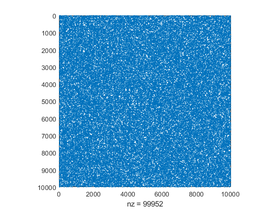
We generate a random sparse matrices of different dimension with sparsity 0.1 per cent. We compare the computing times of our prodK and the mp-package for squaring A:
setround(0)
N = [1000 2000 5000 10000];
for n=N
  A = sprand(n,n,0.001);
  tic
  prodK(A,A,-1,eye(n),2);
  t = toc;
  tic
  double(mp(A)*A - eye(n));
  T = toc;
  fprintf('n = %4d,  t = %4.2f,  T = %4.2f,  T/t = %5.1f\n',n,t,T,T/t)
end
close
spy(A)
n = 1000,  t = 0.14,  T = 0.06,  T/t =   0.4
n = 2000,  t = 0.73,  T = 0.20,  T/t =   0.3
n = 5000,  t = 9.08,  T = 1.33,  T/t =   0.1
n = 10000,  t = 61.51,  T = 5.57,  T/t =   0.1
As can be seen, the highly optimized C-code in the mp-package is about 3 to 10 times as fast as our pure Matlab/Octave implementation.
Next we compare the timing and accuracy of an inclusion of the residual SA-I for an approximate inverse S of A using prodK and the mp-package. Now we choose 1 percent density of A to ensure that A is invertible. Note that the approximate inverse S is full.
N = [1000 2000 5000];
disp([blanks(49) 'median relerr' blanks(7) 'max relerr'])
disp([blanks(49) ' prodK    mp'  blanks(7) ' prodK    mp'])
disp(repmat('-',1,83))
for n=N
  A = sprand(n,n,0.01);
  S = inv(A);
  tic
  [r,e] = prodK(S,A,-1,eye(n),3);
  t = toc;
  tic
  setround(-1)
  Rinf = double(mp(S)*A - eye(n));
  setround(1)
  Rsup = double(mp(S)*A - eye(n));
  T = toc;
  relprodK = relerr(midrad(r,e));
  relmp = relerr(Rinf,Rsup);
  setround(0)
  fprintf('n = %5d, t = %4.2f,  T = %5.2f,  T/t = %4.1f   %8.1e%8.1e   %8.1e%8.1e\n', ...
    n,t,T,T/t,median(relprodK(:)),median(relmp(:)),max(relprodK(:)),max(relmp(:)))
end
                                                 median relerr       max relerr
                                                  prodK    mp        prodK    mp
-----------------------------------------------------------------------------------
n =  1000, t = 0.23,  T =  1.23,  T/t =  5.3    4.2e-14 2.0e-31    1.3e-08 1.3e-29
n =  2000, t = 1.23,  T =  8.41,  T/t =  6.8    1.6e-13 7.9e-31    2.4e-06 2.5e-29
n =  5000, t = 16.43,  T = 111.78,  T/t =  6.8    1.1e-13 6.3e-30    1.5e-06 4.0e-28
The results are of similar accuracy, however, prodK is significantly faster than the mp-package.
Enjoy INTLAB
INTLAB was designed and written by S.M. Rump, head of the Institute for Reliable Computing, Hamburg University of Technology. Suggestions are always welcome to rump (at) tuhh.de