Utility routines
Contents
- Gaussian elimination using naive interval arithmetic
- Gaussian elimination using affine interval arithmetic
- Gaussian elimination using gradients
- Gaussian elimination using hessians
- Gaussian elimination using k-bit arithmetic
- Gaussian elimination over GF[p]
- Random integers
- Even/odd
- Ill-conditioned matrices
- The parity of a permutation
- Positive definiteness of a matrix
- Prove of regularity of matrix with arbitrary condition number
- Full rank of a matrix
- Random orthogonal matrices
- Relative errors
- Distance in bits and the accuracy of inclusion functions
- The bit pattern
- Minimum precision to store data
- Intelligent help
- Greatest common divisor and least common multiple
- All factors of an integer and perfect numbers
- Symbolic computations with pretty output
- Checking exponential many possibilities
- Traversing all vertices of an interval matrix
- Enjoy INTLAB
Gaussian elimination using naive interval arithmetic
The generic routine solvewpp (Solve linear system With Partial Pivoting) works for a number of data types. It is based on Gaussian elimination with subsequent forward and backward substitution using corresponding routines luwpp, forward and backward.
The first example is using ordinary interval arithmetic. The entries of the matrix are afflicted with a relative error of 1e-10.
format long
n = 5;
a = randn(n).*midrad(1,1e-10);
b = a*ones(n,1);

format long
xint = solvewpp(a,b)
intval xint =
   1.00000000______
   1.00000000______
   1.00000000______
   1.00000000______
   1.00000000______
Gaussian elimination using affine interval arithmetic
Next we check whether the result is narrower using affine arithmetic.
xaff = solvewpp(affari(a),b)
[ rad(xint) rad(xaff) ]
intval xaff =
   1.00000000______
   1.00000000______
   1.00000000______
   1.00000000______
   1.00000000______
ans =
   1.0e-08 *
   0.918989773168732   0.918989773168732
   0.115808329592682   0.115808329592682
   0.617540307779052   0.617540307779052
   0.249784382067020   0.249784382067020
   0.303823000091796   0.303823000091796
Gaussian elimination using gradients
We may solve the linear system with gradients as well:
xgra = solvewpp(gradientinit(a),b);
xgra.x
intval ans =
   1.00000000______
   1.00000000______
   1.00000000______
   1.00000000______
   1.00000000______
The data can be used to analyze the sensitivity of individual solution components with respect to individual matrix components. Suppose we want to know how the 3rd solution component depends on the upper left matrix entry a(1,1). The answer is
sens = xgra(3).dx(1)
intval sens =
  -0.7093066_______
This can be verified by direct computation using the midpoint equation:
xs = a.mid\b.mid;
e = 1e-10;
aa = a.mid; aa(1,1) = aa(1,1)+e;
xss = aa\b.mid;
sens_ = ( xss(3)-xs(3) ) / e
sens_ =
  -0.709302616641594
Gaussian elimination using hessians
The linear system can be solved with hessians as well, so that information on all partial second derivatives are available. We only display the second derivative of the 3rd solution components with respect to the upper left matrix element a(1,1).
format short
xhes = solvewpp(hessianinit(a),b);
struct(xhes)
sens_hx = xhes(3).hx(1)
ans =
  struct with fields:

     x: [5×1 intval]
    dx: [25×5 intval]
    hx: [625×5 intval]
intval sens_hx =
  (1,1)                 0.4284
Gaussian elimination using k-bit arithmetic
INTLAB's fl-package uses k-bit IEEE 754 binary arithmetic. After initialization, in this example to 22 bits and exponent range -99 ... 100, Gaussian elimination is performed in this precision.
flinit(22,100)
flinit('DisplayDouble')
xflk = solvewpp(fl(a),b)
ans =
    'Initialization of fl-format to 22 mantissa bits incl. impl. 1 and exponent range -99 .. 100 for normalized fl-numbers'
===> Display fl-variables as doubles
fl-type intval xflk =
    1.0000
    1.0000
    1.0000
    1.0000
    1.0000
Often it is convenient to display the bit pattern of the answer. The format can be changed by
format flbits
xflk
===> Display fl-variables by bit representation
fl-type intval xflk =
 [ +1.111111111111110010101 * 2^-1   , +1.000000000000000110101 * 2^0    ]
 [ +1.111111111111111110100 * 2^-1   , +1.000000000000000000110 * 2^0    ]
 [ +1.111111111111110111000 * 2^-1   , +1.000000000000000100101 * 2^0    ]
 [ +1.111111111111111100011 * 2^-1   , +1.000000000000000001110 * 2^0    ]
 [ +1.111111111111111011011 * 2^-1   , +1.000000000000000010010 * 2^0    ]
Gaussian elimination over GF[p]
INTLAB's gfp-package implements a finite field GF[p] for some prime p. Floating-point numbers are rational and can thus be regarded as elements of a finite field. An example is the inverse over GF[17]:
gfpinit(17)
n = 5;
A = gfp(hilbert(n))
R = solvewpp(A,eye(n))
Galois field prime set to 17
ans =
    17
gfp A =
     4     2     7     1    11
     2     7     1    11    12
     7     1    11    12     3
     1    11    12     3     9
    11    12     3     9     8
gfp R =
     2    10    16     7    13
    10    10     1     5    12
    16     1     6    10    14
     7     5    10     5    16
    13    12    14    16     9
Here hilbert(n) denotes the Hilbert matrix multiplied by the least common multiple of all denominators. Correctness of the computed inverse is verified by
R*A
gfp ans =
     1     0     0     0     0
     0     1     0     0     0
     0     0     1     0     0
     0     0     0     1     0
     0     0     0     0     1
Random integers
Sometimes random integers are needed. Here is how to generate an m x n matrix of integers in the range [1 ... k] or [ -k ... k] .
m = 2;
n = 7;
k = 10;
ipos = randint(k,m,n)
igen = randint(-k,m,n)
ipos =
     7     2     1     5     4    10    10
     6     8     4     2     6    10     2
igen =
     2     0    -4     6    -1    -3    -7
    10    -2    10     4     0    -1    -3
Even/odd
Sometimes it may be useful to check the parity of an integer. As the name suggests, odd(n) is 1 for odd n. It may be applied to a vector as well.
N = randint(-10,1,5)
Nodd = odd(N)
Neven = even(N)
Nodd | Neven
N =
     8     8    -4    -7    -3
Nodd =
  1×5 logical array
   0   0   0   1   1
Neven =
  1×5 logical array
   1   1   1   0   0
ans =
  1×5 logical array
   1   1   1   1   1
Ill-conditioned matrices
The routine randmat generates extremely ill-conditioned matrices.
n = 50;
cnd = 1e25;
A = randmat(n,cnd);
c = cond(A)
c =
   5.5470e+17
Of course, the Matlab routine cond cannot approximate the true condition number of about cnd=1e25. The true condition number can be computed by INTLAB's especially designed inclusion algorithm for extreme condition numbers (up to about 1e30).
C = cond(intval(A),'illco')
intval C =
  1.0e+022 *
    6.3794
Note that C is an inclusion of the true 2-norm condition number.
The parity of a permutation
Mathematically, independent of the matrix B, the matrix A computed by
n = 5;
B = boothroyd(n)/10;
A = B'*B
A =
   1.0e+03 *
    0.2225    0.7292    0.9277    0.5373    0.1187
    0.7292    2.3930    3.0465    1.7650    0.3902
    0.9277    3.0465    3.8800    2.2485    0.4973
    0.5373    1.7650    2.2485    1.3033    0.2883
    0.1187    0.3902    0.4973    0.2883    0.0638
must be positive semi-definite. However, due to rounding errors it might not. The method of choice to factor A would be Cholesky decomposition. However, Gaussian elemination may produce a permutation although mathematically not necessary:
[L,U,p] = lu(A,'vector')
L =
    1.0000         0         0         0         0
    0.7860    1.0000         0         0         0
    0.2398    0.8511    1.0000         0         0
    0.5791   -0.4832    0.3932    1.0000         0
    0.1280   -0.1829    0.1851    0.5220    1.0000
U =
   1.0e+03 *
    0.9277    3.0465    3.8800    2.2485    0.4973
         0   -0.0017   -0.0033   -0.0024   -0.0006
         0         0    0.0000    0.0000    0.0000
         0         0         0    0.0000    0.0000
         0         0         0         0    0.0000
p =
     3     2     1     4     5
To verify that, at least numerically, the determinant of A is not negative the parity is used:
d = prod(diag(U))
par = parity(p)
d =
  -1.0000e-10
par =
    -1
Positive definiteness of a matrix
The following verifies rigorously that the matrix A of the previous example is indeed positive definite:
isspd(A)
ans =
  logical
   1
Prove of regularity of matrix with arbitrary condition number
Based on number theory and mod(p) calculations it is possible to verify the regularity of arbitrarily ill-conditioned matrices in short computing time. If, by chance, the test should not work, a second parameter specifying a kind of probability is possible.
An example with extreme condition number of about 1e100 is as follows.
n = 200;
cnd = 1e100;
A = randmat(n,cnd);
tic
reg = isregular(A)
T = toc
reg =
     1
T =
    0.1106
Note that the proof of regularity is rigorous. As is well-known, a proof of singularity in the same manner is an ill-posed problem.
Full rank of a matrix
Similarly it can be verified that a rectangular matrix has full rank. An answer 1 proves that the matrix has full rank. If the following
A = randn(5,3)*rand(3,5)
A =
    2.6220    0.3689    2.5148    0.8257    0.4400
    0.8321    0.5453    0.9505    0.6471    0.5835
   -1.8620   -1.4494   -1.9208   -1.5629   -1.2682
   -0.9545   -0.0272   -0.5892   -0.1129    0.2263
    0.0288   -0.5806   -0.2912   -0.5518   -0.7071
is computed in real arithmetic, the result matrix A has at most rank 3. However, due to rounding errors the result has full rank:
isfullrank(A)
ans =
     1
For integer input no rounding error occur and the resulting matrix is indeed rank-deficient:
A = randint(-10,5,3)*randint(-10,3,5)
isfullrank(A)
A =
    90   -71    50    85    63
    40   -19    26    43    25
   -62    41   -34   -60   -44
   -82    13   -26   -76   -76
   -18    31   -34   -29     9
ans =
     0
Here randint(-10,5,3) produces a 5x3 matrix with random integers in [-10,10]. The rank-deficiency of A in some Galois field can be verified:
gfpinit(67108859)
[L,U,p,q,growth,r] = luwtp(gfp(A))
Galois field prime set to 67108859
ans =
    67108859
gfp L =
           1           0           0           0           0
    67108854           1           0           0           0
    37282704    26719267           1           0           0
    29826163      124275    13421772           1           0
    52195777     1615584    40265315           0           1
gfp U =
    67108841    67108830           9          31    67108825
           0    67108799         108          84    67108739
           0           0    67108843    22369570    44739256
           0           0           0           0           0
           0           0           0           0           0
p =
     5     1     4     3     2
q =
     1     4     5     2     3
growth =
     1
r =
     3
Mathematically it is shown that A has rank 3 over GF[p], it might have a higher rank over R.
Random orthogonal matrices
One way to generate matrices with specified singular values uses random orthogonal matrices.
n = 100;
Q = randorth(n);
norm(Q'*Q-eye(n),inf)
ans =
   1.7217e-14
Relative errors
Displaying relative errors has well-known drawbacks. First, there is the problem of numbers near zero: For x=1e-20, is x+1e-25 nearby? Second, the relative error depends on how close a number is to the next power of 2, and whether it is slightly smaller or larger.
The predecessor and successor of 1 and the relative error to 1 is computed by
succ1 = succ(1)
pred1 = pred(1)
relsucc = relerr(1,succ1)
relpred = relerr(1,pred1)
succ1 =
    1.0000
pred1 =
    1.0000
relsucc =
   2.2204e-16
relpred =
   1.1102e-16
Distance in bits and the accuracy of inclusion functions
For very narrow intervals it might sometimes be simpler to use the distance in bits:
distsucc = distbits(1,succ1)
distpred = distbits(1,pred1)
distsucc =
     1
distpred =
    -1
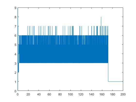
For performance reasons the maximum distance in bits is restricted to 100. The function distbits can be used to track the accuracy of computed inclusions:
 x = linspace(0,200,1e6);
 Y = gamma(intval(x));
 close, plot(x,distbits(Y))
The bit pattern
Also the bit pattern is sometimes useful:
getbits([pred1 1 succ1])
ans =
  3×63 char array
    ' +1.1111111111111111111111111111111111111111111111111111 * 2^-1'
    ' +1.0000000000000000000000000000000000000000000000000000 * 2^0 '
    ' +1.0000000000000000000000000000000000000000000000000001 * 2^0 '
The function applies to intervals as well. It can be used to verify that the bounds are indeed as close as possible:
Pi = intval('pi')
getbits(Pi)
distbits(Pi)
intval Pi =
    3.1415
ans =
  4×62 char array
    'infimum                                                       '
    ' +1.1001001000011111101101010100010001000010110100011000 * 2^1'
    'supremum                                                      '
    ' +1.1001001000011111101101010100010001000010110100011001 * 2^1'
ans =
     1
Displaying bits applies to single precision numbers or the INTLAB fl-toolbox as well:
getbits(single(pi))
flinit(7,50);
getbits(fl(5))
getbits(fl(infsup(11,13)))
ans =
    ' +1.10010010000111111011011 * 2^1'
ans =
    ' +1.010000 * 2^2'
ans =
  4×16 char array
    'infimum         '
    ' +1.011000 * 2^3'
    'supremum        '
    ' +1.101000 * 2^3'
Minimum precision to store data
Sometimes it is convenient to know the minimum necessary precision to store a floating-number. For example
x = single(3.375)
getbits(x)
p = minprec(x)
x =
  single
    3.3750
ans =
    ' +1.10110000000000000000000 * 2^1'
p =
     5
The best approximation for x=0.3 requires 53 bits:
x = 0.3
getbits(x)
minprec(x)
x =
    0.3000
ans =
    ' +1.0011001100110011001100110011001100110011001100110011 * 2^-2'
ans =
    53
Here p=5 shows that x requires at least 5 bits to be stored without rounding error. That includes the implicit 1.
Intelligent help
Sometimes it is not clear how to spell a name and/or we know only parts of a function name, and even that is uncertain. In that case sometimes helpp, an intelligent help function, may be useful. After initialization by just calling "helpp" the following may be obtained:
helpp tschebischeff
ans =
  6×90 char array
    'level 6  C:\intlab versions\intlab\intval\checkrounding.m                                 '
    'level 6  C:\intlab versions\intlab\intval\verifyschur.m                                   '
    'level 6  C:\intlab versions\intlab\intval\@intval\schur.m                                 '
    'level 6  C:\intlab versions\intlab\utility\Fletcher.m                                     '
    'level 9  C:\intlab versions\intlab\polynom\chebyshev.m                                    '
    'level 9  C:\intlab versions\intlab\polynom\chebyshev2.m                                   '
The answer comes with certain levels representing some kind of distance. Sometimes even gross misspelling still retrieves the correct name. Needless to say that it works the better the longer the string to look for.
Greatest common divisor and least common multiple
The smallest common denominator of rational number is the least common multiple of the denominators. For example
lcmvec([12 15 36])
ans =
   180
Correspondingly, greatest common divisor is computed:
v = [12 15 36]
g = gcdvec(v)
v =
    12    15    36
g =
     3
All factors of an integer and perfect numbers
The list of all factors of an integer is computed by
factors(123456789)
ans =
  Columns 1 through 6
           1           3           9        3607        3803       10821
  Columns 7 through 11
       11409       32463       34227    13717421    41152263
It can be used to verify that a number is perfect:
n = 28
f = factors(n)
sum(f)
n =
    28
f =
     1     2     4     7    14
ans =
    28
Symbolic computations with pretty output
The pretty output of symbolic expressions is often useful:
syms x
P = 1;
for i=1:5
  P = P * (x^2-i);
end
pretty(collect(P,x))
 10       8       6        4        2
x   - 15 x  + 85 x  - 225 x  + 274 x  - 120
However, the statement leading to the pretty output is not visible. That can be done as follows:
pretty('collect(P,x)')
collect(P,x) =
 10       8       6        4        2
x   - 15 x  + 85 x  - 225 x  + 274 x  - 120
Checking exponential many possibilities
Given an interval matrix A it is known to be an NP-hard problem to verify non-singularity. The best criterion known still needs 2^n steps for a given n x n matrix. The result is as follows:
Theorem (Rohn). A given interval matrix mA +/- r*E for E denoting the matrix of all 1's, is non-singular if and only if r < 1/sum(abs(inv(A)*x)) for all vectors x with components +/-1 .
The maximum quantity r is the so-called radius of non-singularity. Compared to checking all vertices the theorem reduces the number of determinants from 2^(n^2) to 2^n.
The function bin2vec is useful to generate all signature matrices. The call v = bin2vec(i,n) generates the vector of the n least significant bits of i.
n = 4;
A = hadamard(n)
Ainv = inv(A);
R = 0;
for i=1:2^n
  x = (2*bin2vec(i,n)-1)';
  r = sum(abs( Ainv * x ));
  if r>R, R=r; end
end
singRad = 1/R
A =
     1     1     1     1
     1    -1     1    -1
     1     1    -1    -1
     1    -1    -1     1
singRad =
    0.5000
Traversing all vertices of an interval matrix
The function bin2vec can also be used to visit all vertices of an interval matrix. These are, however, 2^(n^2) vertices. With the method before we checked that the radius of non-singularity of the 8x8 Hadamard matrix is 0.5. Thus A=midrad(hadamard,0.499) must be non-singular. This is checked as follows.
tic
n = 4;
A = hadamard(n);
s = sign(det(A));
for i=1:2^(n^2)
  D = det( A + 0.499*reshape( 2*bin2vec(i,n^2)-1 , n,n ) );
  if D*s<0
    disp('The interval matrix is singular')
    break
  end
end
if D*s>0
  disp('The interval matrix is non-singular')
end
T = toc
The interval matrix is non-singular
T =
    0.0528
The function v = base2vec(i,b,n) does the same for base b.
Enjoy INTLAB
INTLAB was designed and written by S.M. Rump, head of the Institute for Reliable Computing, Hamburg University of Technology. Suggestions are always welcome to rump (at) tuhh.de