DEMOTAYLORMODEL Short demonstration of the Taylor model toolbox

This toolbox is a MATLAB/INTLAB-implementation of the Taylor model approach for solving ODEs with mathematically rigorous results. For details on that approach we refer to the references at the end. The main function is the ODE solver verifyode.

In principle, Taylor models are, like intervals, objects on their own which may serve for various other kinds of verified computations. We emphasize that this toolbox is not designed for such general applications of Taylor models. It is deliberately focused on ODEs.

The routine verifyode creates all Taylor models automatically, basically hidden from a user. In principle, the user does not even need to know what Taylor models are. Nevertheless, the first two sections give some brief technical insight into their definition and arithmetic. Users who are not interested in those details may directly proceed to Section "verifyode - Syntax".

Definition of Taylor models
Taylor model arithmetic
verifyode - Syntax
Description
Introductory example
Example II - Lotka-Volterra equations, a two-dimensional ODE system
Example III - The Lorenz system
Example IV - The van der Pol equation, a second order ODE
Example V - A quadratic model problem
Example VI - A Kepler problem for asteroid motion
Input Arguments
Output Arguments
Display results
References
Enjoy INTLAB

Definition of Taylor models

The simplest way is to think of a Taylor model as a multivariate, real polynomial p of bounded degree d in a fixed number of n variables. Such a polynomial is usually written as

$p(x) = \sum_{a,|a|\leq d} p_{a} x^a, \quad |a| := a_1 + ... + a_n, \quad x^a := x_1^{a_1} \cdots x_n^{a_n},$

where a = (a_1,...,a_n) is a multi index consisting of non negative integer exponents a_i and the polynomial coefficients p_a are real numbers. Now, an n-dimensional domain

$D = [u_1,v_1] \times \dots \times [u_n,v_n]$

is fixed which is simply an interval vector of length n with interval components [u_i,v_i], i = 1,...,n. Next, a "center point" c = (c_1,...,c_n) in D is fixed which must not necessarily be the exact center (u+v)/2. For example, c = u or c = v are also allowed, only c_i must be in [u_i,v_i]. The standard domain and center point are

$Ds := [-1,1] \times \dots \times [-1,1], \quad cs := (0,...,0).$

The centered image

$p(D-c) = \{ p(x-c) ~|~ x \in D \}$

is the enclosure represented by the data p, D, and c. For the special case of degree d = 1, standard domain Ds, and center point cs this coincides with the enclosure represented by an object in affine arithmetic with n error terms.

Moreover, a Taylor model contains an error interval E which absorbs the inevitable rounding and degree truncation errors. Thus, the enclosure (range) represented by the Taylor model data p, D, c, E enlarges to

$p(D-c) + E = \{p(x-c) + e ~|~ x \in D, e \in E\}.$

We remark that the polynomial coefficients p_a, the domain bounds u_i, v_i, and the center points c_i are restricted to be floating-point numbers in order to keep them representable on a computer.

For the single Taylor model y = (p,D,c,E) the range is a closed interval. In particular, it is convex. Taking a second Taylor model z = (q,D,c,F) with same domain and center point, the range R of the Taylor model vector w = (y,z) is defined by

$R = \{(p(x-c) + e, q(x-c) + f) ~|~ x \in D, e \in E, f \in F\}.$

This set R is not necessarily convex anymore. This is the big advantage of Taylor models: they allow to enclose higher dimensional shapes with curved boundaries without too much overestimation, see the pictures in Section "Taylor model arithmetic".

As a first simple example, a Taylor model y with polynomial part

$p(x_1,x_2) = 2 + x_1 - x_2 + 3x_1^2x_2^3$

of degree d = 5, standard domain, standard center point, and error interval [-1e-6,1e-6] can be created as follows:

p = [2;1;-1;3];  % polynomial coefficients
M = [0 0;        % polynomial exponents
     1 0;
     0 1;
     2 3];
order = 7;       % some degree bound >= d
D.inf = [-1;-1]; % lower domain bounds
D.sup = [1;1];   % upper domain bounds
c = [0;0];       % center point
E.inf = -1e-6;
E.sup = 1e-6;
format shortg infsup
y = taylormodelinit(c,D,order,M,p,E)

taylormodel y = 
 
    dim    order    type    iv_mid    iv_rad    im_inf    im_sup
    ___    _____    ____    ______    ______    ______    ______
     2       7       0        0       1e-06       -3        7   
 
          min    max    center
          ___    ___    ______
    x1    -1      1       0   
    x2    -1      1       0   
 
    x1    x2    coeff
    __    __    _____
    0     0       2  
    1     0       1  
    0     1      -1  
    2     3       3

A quite large enclosure [im_inf,im_sup] = [-3,7] of the polynomial image p(D-c) = p(D) = [-3,5] is computed automatically. The true range R = [-3,5] + E of y is very much overestimated by [-3,7] + E. In practice, Taylor models with thin ranges of diameter much less than 1 are typical. Only for ease of presentation we chose the stated data with wide range.

Technically, the components of a Taylor model read as follows:

ys = struct(y)
ys_dim = ys.dim                             % number of unknowns
ys_center = ys.center                       % center point c
ys_domain = [ys.domain.inf,ys.domain.sup]   % domain D
ys_order = ys.order                         % degree bound
ys_monomial = ys.monomial                   % polynomial exponents
ys_coefficient = ys.coefficient             % polynomial coefficients p
ys_interval = ys.interval                   % error interval E
ys_type = ys.type                           % Taylor model type
ys_image = ys.image                         % enclosure of polynomial image p(D-c)

ys = 
  struct with fields:

            dim: 2
         center: [2×1 double]
         domain: [1×1 struct]
          order: 7
       monomial: [4×2 double]
    coefficient: [4×1 double]
       interval: [1×1 struct]
           type: 0
          image: [1×1 struct]
ys_dim =
     2
ys_center =
     0
     0
ys_domain =
    -1     1
    -1     1
ys_order =
     7
ys_monomial =
     0     0
     1     0
     0     1
     2     3
ys_coefficient =
     2
     1
    -1
     3
ys_interval = 
  struct with fields:

    inf: -1e-06
    sup: 1e-06
ys_type =
     0
ys_image = 
  struct with fields:

    inf: -3
    sup: 7

Taylor models of type 0 are the default, Taylor models of type 1 are used for solving ODEs. The latter have special domains and center points of the form

$D = [-1,1]\times \dots \times [-1,1] \times [t_1,t_2], \quad c = (0,\dots,0,t_1)$

where [t_1,t_2] is the time domain, i.e., the domain of the variable t with respect to which the integration is performed from t_1 to t_2.

Taylor model arithmetic

Similar to affine arithmetic, a strength of Taylor model arithmetic lies in respecting dependencies of the input data. For simplicity, let us consider the Taylor model y from above with zero error interval

y = taylormodelinit(c,D,order,M,p);

and its true range

R = infsup(-3,5)

intval R = 
[   -3.0000,    5.0000]

Then,

a = y - y
b = R - R

taylormodel a = 
 
    dim    order    type    iv_mid    iv_rad    im_inf    im_sup
    ___    _____    ____    ______    ______    ______    ______
     2       7       0        0         0         0         0   
 
          min    max    center
          ___    ___    ______
    x1    -1      1       0   
    x2    -1      1       0   
 
    x1    x2    coeff
    __    __    _____
    0     0       0  
intval b = 
[   -8.0000,    8.0000]

shows that the Taylor model result a = 0 with the range [im_inf,im_sup] = {0} is mathematically exact, while traditional interval arithmetic produces b = [-8,8] due to ignoring data dependencies in the expression R-R. For the trivial case of a single interval, the result of affine arithmetic is zero, the same as the Taylor model result:

R_ = affari(R)
b_ = R_ - R_

affari R_ = 
[   -3.0000,    5.0000] 
affari b_ = 
[    0.0000,    0.0000]

Let us now consider a second Taylor model z with polynomial part $q = 3 - x_1^2x_2^3$ :

q = [3;-1]; % polynomial coefficients
N = [0 0;   % polynomial exponents
     2 3];
z = taylormodelinit(c,D,order,N,q);

Clearly,

$p+q = 5 + x_1 - x_2 + 2x_1^2x_2^3$

is the polynomial part of r_plus := y+z:

r_plus = y+z

taylormodel r_plus = 
 
    dim    order    type    iv_mid    iv_rad    im_inf    im_sup
    ___    _____    ____    ______    ______    ______    ______
     2       7       0        0         0         1         9   
 
          min    max    center
          ___    ___    ______
    x1    -1      1       0   
    x2    -1      1       0   
 
    x1    x2    coeff
    __    __    _____
    0     0       5  
    1     0       1  
    0     1      -1  
    2     3       2

Note that no rounding errors occur in the summation of the polynomial coefficients wherefore the error interval of the Taylor model result r_plus stays zero.

At first glance surprising, the polynomial part of the product r_mult := y*z is not

$pq = 6 + 3x_1 - 3x_2 + 7x_1^2x_2^3 + x_1^2x_2^4 - x_1^3x_2^3 - 3x_1^4x_2^6$

but only the part of order up to the degree bound 7. This is

$s := 6 + 3x_1 - 3x_2+ 7x_1^2x_2^3+ x_1^2x_2^4 - x_1^3x_2^3$

The image [-3,0] = midrad(-1.5,1.5) of the truncated term $-3x_1^4x_2^6$ of degree 10 moves to the error interval of r_mult.

r_mult = y*z

taylormodel r_mult = 
 
    dim    order    type    iv_mid    iv_rad    im_inf    im_sup
    ___    _____    ____    ______    ______    ______    ______
     2       7       0       -1.5      1.5        -8        21  
 
          min    max    center
          ___    ___    ______
    x1    -1      1       0   
    x2    -1      1       0   
 
    x1    x2    coeff
    __    __    _____
    0     0       6  
    1     0       3  
    0     1      -3  
    2     3       7  
    3     3      -1  
    2     4       1

Having summation and multiplication at hand, unary standard functions like exp, log, sin, cos, etc. for Taylor models can be defined through finite Taylor series expansions of those functions and bounding the remainder term in a verified manner. This procedure coined the name "Taylor models". For details we refer to the references [E] and [M] below.

As stated in Section "Definition of Taylor models", the main advantage of Taylor models is that they allow to enclose multidimensional shapes with curved, not necessarily convex boundaries and without too much overestimation. This is not possible for traditional interval arithmetic which only supplies enclosures in axis parallel boxes. It is also not possible for affine arithmetic which only provides convex polytopes as enclosure sets.

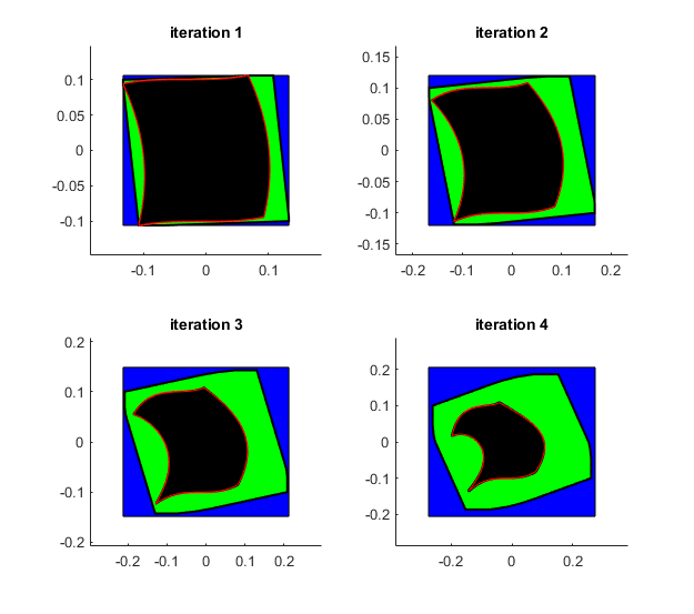
As an example let us consider the square B = [-r,r] x [-r,r] with r = 0.1, which shall be mapped iteratively by the function

$f(x,y) = ( \; x - y(0.125 + 2y) \; , \; y + 6x^3 \; ) .$

The following program executes four such iterations with

interval arithmetic (blue plot)
affine arithmetic (green plot)
Taylor model arithmetic (black plot)

For each iteration the curved red line shows the approximate true boundary of the transformed box B, i.e., the boundary of the sets f(B), f(f(B)), f(f(f(B))), and f(f(f(f(B)))), respectively. The four pictures clearly show that Taylor model arithmetic creates almost no overestimation compared to the rough inclusions supplied by interval arithmetic and affine arithmetic.

f = @(x,y) [ x - y.*(0.125 + 2*y) , y + 6*x.^3 ];
r = 0.1;
B = midrad([0;0],r);         % interval representation of B = [-r,r]x[-r,r]
a = (-1:0.01:1)';
e = ones(length(a),1);
b = r*[a e;e -a;-a -e;-e a]; % discretized boundary of B
y_fl = b;
y_iv = B;
y_af = affari(B);            % affine arithmetic representation of B
y_tm = taylormodelinit({c;c},{D;D},[18;18],{[1 0];[0 1]},{r;r});
                             % Taylor model representation of B (order = 18)
close all
for i = 1:4
  subplot(2,2,i)
  title(['iteration ', num2str(i)])
  hold on
  y_iv = f(y_iv(1),y_iv(2));      % Evaluate f in interval arithmetic
  plotintval(y_iv','b');          % ... and plot the enclosure in blue.
  y_af = f(y_af(1),y_af(2));      % Evaluate f in affine arithmetic
  plotaffari(y_af','g');          % ... and plot the enclosure in green.
  y_tm = f(y_tm(1),y_tm(2));      % Evaluate f in Taylor model arithmetic
  plottaylormodel(y_tm,[],[],100) % ... and plot the enclosure in black.
  y_fl = f(y_fl(:,1),y_fl(:,2));  % Compute approximate boundary of f(f(...(B)))
  plot(y_fl(:,1),y_fl(:,2),'r');  % ... and plot it as red line.
end
set(gcf, 'Units', 'Normalized', 
'OuterPosition', [0 0 0.5 0.8]);
hold off

verifyode - Syntax

Calling verifyode is similar to calling a MATLAB ODE solver like ode45:

[T,Y] = verifyode(odefun,tspan,y0)
[T,Y] = verifyode(odefun,tspan,y0,options)
[T,Y,Yr] = verifyode(odefun,tspan,y0,options)

Description

[T,Y] = verifyode(odefun,tspan,y0), where tspan = [t0 tf], integrates the system of differential equations y' = f(t,y) from t0 to tf with initial conditions y0. (Integration in negative direction, i.e., tf < t0 is supported.) Each row of the Taylor model array Y represents an inclusion of the solution y on a time interval of the time grid T. The time grid T is simply a floating-point column vector of time grid points T(i) where T(1) = t0 and T(m) = tf, m = length(T). Precisely, for t in [T(j),T(j+1)] the solution y(t) at time t is contained in the set

$Y_j(t) = \{ (p_1(x,t)+e_1,\dots,p_n(x,t)+e_n)~|~ x \in [-1,1]^n, e_i \in E_i, i=1,\dots,n \}$

where n is the dimension of the ODE, p_i is the polynomial part and E_i is the error interval of the Taylor model Y(j,i), j = 1,..,m-1, i = 1,...,n.

The initial condition y0 may be an interval vector. In that case the computed inclusion Y contains the true solution of the differential equation for any initial values y_i(t0) in the interval y0(i), i = 1,...,n. This allows to model uncertainties in the initial values.

As demonstrated in the previous section, Taylor models are especially well-suited for enclosing multidimensional shapes with curved boundary. Such shapes occur naturally in flows of nonlinear ODE systems (n >= 2) with interval initial conditions, where at time s the initial interval box y0 is transformed to the set

$\{ y(s) ~|~ y' = f(t,y), \ y(t_0) \in y0\}.$

Taylor model arithmetic of high order is expensive. Thus, for solving ODE systems with point initial conditions, other verified ODE solvers like awa might be tried first because, in general, they run much faster.

Concluding this section, we remark that the right-hand side f(t,y) of the ODE must be implemented by the user. It is passed to verifyode by a corresponding function handle odefun, see the detailed description in Section "Input Arguments".

Introductory example

Solve the ODE

$y' = \frac{1}{2} \cdot y \ .$

Use a time interval [0,2] and the initial condition y0 = 1.

tspan = [0,2];
y0 = 1;
lambda = 0.5;
odefun = @(t,y,i) lambda.*y;        % odefun must accept three inputs (t,y,i) even though t and i are not used.
[T,Y] = verifyode(odefun,tspan,y0);

The function verifyode_disp can be used to display enclosures at all time grid points:

format long e
verifyode_disp(T,Y,[],y0);

t = 0
    [y] = [  1.000000000000000e+000,  1.000000000000000e+000]    d([y]) = 0.00e+00
 
t = 1.259155104576573e-01
    [y] = [  1.064981848366509e+000,  1.064981848366514e+000]    d([y]) = 3.11e-15
 
t = 3.760579115397761e-01
    [y] = [  1.206868460649098e+000,  1.206868460649105e+000]    d([y]) = 5.77e-15
 
t = 8.678986551468919e-01
    [y] = [  1.543340661318726e+000,  1.543340661318739e+000]    d([y]) = 1.07e-14
 
t = 1.805635813523891e+00
    [y] = [  2.466543817935057e+000,  2.466543817935110e+000]    d([y]) = 4.97e-14
 
t = 2
    [y] = [  2.718281828459015e+000,  2.718281828459076e+000]    d([y]) = 6.04e-14

For example, at the final grid point t = 2 the solution y(t) = y(2) = exp(1) is contained in the interval

[y] = [2.718281828459015e+000, 2.718281828459076e+000]

with diameter d([y]) = 6.04e-14. For comparison we may use the intval exponential directly:

exp1 = exp(intval(1))

intval exp1 = 
[  2.718281828459043e+000,  2.718281828459047e+000]

The function verifyode_disp can also compute and display verified enclosures at arbitrary (floating-point) time points in [0,2]. For example,

x = 2*rand
format long _
[t,y] = verifyode_disp(T,Y,[],y0,x);
incl = in(exp(intval(x)/2),y) % Check whether INTLAB's interval enclosure of exp(x/2) is contained in the verifyode enclosure y.

x =
     5.077469341958626e-01
t = 0.507746934195863
    [y] = [   1.28900869193789,   1.28900869193791]    d([y]) = 1.07e-14
 
incl =
  logical
   1

returns and displays an interval enclosure at the randomly chosen t = x which is surely not a grid point in T. [The formatted display is suppressed by calling [t,y] = verifyode_disp(T,Y,[],y0,x,false).]

Also enclosures for time intervals that are contained in [0,2] can be computed in that way. For example,

x = intval('pi')/2
[t,y] = verifyode_disp(T,Y,[],y0,x);
incl = in(exp(x/2),y) % Check whether INTLAB's interval enclosure of exp(x/2) = exp(pi/4) is contained in the verifyode enclosure y.

intval x = 
   1.57079632679489
t = 1.57079632679489
    [y] = [   2.19328005073800,   2.19328005073806]    d([y]) = 4.97e-14
 
incl =
  logical
   1

returns and displays an interval enclosure at t = $\pi$ /2. Here INTLAB's command x = intval('pi')/2 is used to calculate an inclusion of $\pi$ /2, which is not a floating-point number, in an interval x. Afterwards, verifyode_disp computes an enclosure which is valid at all time points of x, especially at t = $\pi$ /2.

A previous integration can also be continued. For example, if integration shall be resumed from tf_old = 2 up to tf_new = 4, then this is done as follows:

tf_new = 4;
[T_new,Y_new] = verifyode(odefun,tf_new,{T,Y});
[t,y] = verifyode_disp(T_new,Y_new,[],y0,tf_new);
incl = in(exp(intval(2)),y) % Check whether INTLAB's interval enclosure of exp(2) = exp(tf_new/2) is contained in the verifyode enclosure y.

t = 4
    [y] = [   7.38905609893049,   7.38905609893085]    d([y]) = 3.47e-13
 
incl =
  logical
   1

The new end time tf_new = 4 and the result {T,Y} of the previous run, which shall be continued, are passed to the function verifyode in the input arguments tspan = tf_new and y0 = {T,Y}, respectively. Then, verifyode automatically detects the old end time tf_old = 2 from which it starts. Finally, the new result T_new, Y_new contains the data for the whole integration period [0,tf_new] = [0,4]. [Additional parameter settings specified in the input argument "options" of verifyode, see Section "Input arguments", must stay the same. If preconditioning is switched on, then {T,Y,Yr} (and not only {T,Y}) must be passed, see Section "Output arguments".]

Furthermore, integration can be done in negative direction. For example, backward integration from t0 = 0 to tf = -2 is done as follows:

[T,Y] = verifyode(odefun,[0,-2],y0);
format long e
verifyode_disp(T,Y,[],y0);
[t,y] = verifyode_disp(T,Y,[],y0,-2);
incl = in(exp(intval(-1)),y) % Check whether INTLAB's interval enclosure of exp(-1) = exp(tf/2) is contained in the verifyode enclosure y.

t = 0
    [y] = [  1.000000000000000e+000,  1.000000000000000e+000]    d([y]) = 0.00e+00
 
t = -1.259155104576573e-01
    [y] = [  9.389831399791622e-001,  9.389831399791639e-001]    d([y]) = 1.44e-15
 
t = -3.897570822502702e-01
    [y] = [  8.229346046973648e-001,  8.229346046973678e-001]    d([y]) = 2.78e-15
 
t = -9.367089493606768e-01
    [y] = [  6.260315719803931e-001,  6.260315719803986e-001]    d([y]) = 5.22e-15
 
t = -1.681012684808203e+00
    [y] = [  4.314919854169666e-001,  4.314919854169762e-001]    d([y]) = 9.38e-15
 
t = -2
    [y] = [  3.678794411714368e-001,  3.678794411714487e-001]    d([y]) = 1.18e-14
 
t = -2
    [y] = [  3.678794411714368e-001,  3.678794411714487e-001]    d([y]) = 1.18e-14
 
incl =
  logical
   1

Example II - Lotka-Volterra equations, a two-dimensional ODE system

The well-known Lotka-Volterra equations read:

$\begin{array}{ccl} y'_1 &=& 2 y_1 (1-y_2) \ , \\ y'_2 &=& y_2 (y_1-1) \ . \end{array}$

The function file lotka_volterra.m implements these equations.

function dydt = lotka_volterra(t,y,i)
  if nargin == 2 || isempty(i)
    dydt = [2.*y(1).*(1-y(2));    % y1' = 2*y1*(1-y2)
            (y(1)-1).*y(2)];      % y2' = (y1-1)*y2
  else
    switch i
      case 1                      % Compute only first component.
        dydt = 2.*y(1).*(1-y(2));
      case 2                      % Compute only second component.
        dydt = (y(1)-1).*y(2);
    end
  end

The third input argument i allows to compute specific function components separately. This was invented to improve the performance of verifyode since Taylor model arithmetic is expensive.

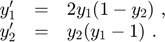
The ODE shall be solved on the time interval [0,5.5] (which covers a full predator-prey cycle modeled by the system) with interval initial values y_0 = [0.95,1.05]x[2.95,3.05], see [MB1], and [E], Chapter 5. The resulting output is a floating-point column vector of time points T and a solution Taylor model array Y. Each row j in Y corresponds to a time interval [T(j),T(j+1)]. The first column of Y contains Taylor models for y_1, and the second column for y_2.

We use the function verifyodeset to set some options for verifyode. This is similar to MATLAB's function odeset. In particular preconditioning is switched on which generates the third output argument Yr (right Taylor models). See the detailed description of possible options in Section "Input Arguments".

t0 = 0;                  % start time
tf = 5.5;                % end time
y0 = midrad([1;3],0.05); % interval initial conditions
options = verifyodeset('order',18, 'shrinkwrap',false, 'precondition',1, 'blunting',false,...
                       'h0',0.03, 'h_min',0.003, 'loc_err_tol',1e-11, 'sparsity_tol',1e-20);
tic
[T,Y,Yr] = verifyode(@lotka_volterra,[t0,tf],y0,options);
toc

Elapsed time is 4.089485 seconds.

The enclosures for y_1 and y_2 are plotted against t by using INTLAB's plot function. For comparison, the system is also solved with ode45 for initial conditions y0.inf = [1.95;2.95] and y0.sup = [2.05;3.05]. First, ode45 uses its default options. The two results are stored in [t_inf,v_inf] and [t_sup,v_sup]. Second, ode45 is executed with higher accuracy and the results are stored in [s_inf,w_inf] and [s_sup,w_sup]. The inclusion computed by verifyode and the ode45 approximations are displayed in one plot, the latter in blue and green. The specified value 1e-14 for 'RelTol' in the ode45 options is automatically increased by MATLAB to the minimum relative tolerance 2.22045e-14.

format short
verifyode_disp(T,Y,Yr,y0,tf);                                  % Display enclosure of y at t = tf = 5.5.
tt = linspace(t0,tf,300);                                      % fine grid for plotting
[t,y] = verifyode_disp(T,Y,Yr,y0,tt,false);                    % Compute interval enclosures at fine grid.
figure
plot(t,y)                                                      % Plot enclosures for y_1 and y_2.
title('Solution of Lotka-Volterra Equations with verifyode');
xlabel('Time t')
ylabel('Solution y')
hold on
[t_inf,v_inf] = ode45(@lotka_volterra,tt,y0.inf);              % Execute ode45 with initial condition y0.inf = [1.95;2.95]
[t_sup,v_sup] = ode45(@lotka_volterra,tt,y0.sup);              % Execute ode45 with initial condition y0.sup = [2.05;3.05]
plot(t_inf,v_inf,'.-b',t_sup,v_sup,'.-b')                      % Plot ode45 results as blue lines where grid points are marked as dots.
options = odeset('RelTol',1e-14,'AbsTol',[1e-14 1e-14]);       % Set options for higher accuracy of ode45.
all_in_vinf_y = all(in(v_inf,y))                               % Check whether the ode45 results v_inf and v_sup are contained in the verifyode enclosure y.
all_in_vsup_y = all(in(v_sup,y))
[s_inf,w_inf] = ode45(@lotka_volterra,tt,y0.inf,options);      % Execute ode45 again with higher accuracy.
[s_sup,w_sup] = ode45(@lotka_volterra,tt,y0.sup,options);
all_in_winf_y = all(in(w_inf,y))                               % Check whether the ode45 results w_inf and w_sup are contained in the verifyode enclosure y.
all_in_wsup_y = all(in(w_sup,y))
plot(s_inf,w_inf,'.-g',s_sup,w_sup,'.-g')                      % Plot new ode45 results as green lines where grid points are marked as dots.
hold off

t = 5.5000
    [y_1] = [    0.7801,    1.1818]    d([y_1]) = 4.02e-01
    [y_2] = [    2.9294,    3.0493]    d([y_2]) = 1.20e-01
 
all_in_vinf_y =
  1×2 logical array
   0   0
all_in_vsup_y =
  1×2 logical array
   0   0
Warning: RelTol has been increased to 2.22045e-14. 
Warning: RelTol has been increased to 2.22045e-14. 
all_in_winf_y =
  1×2 logical array
   1   1
all_in_wsup_y =
  1×2 logical array
   1   1

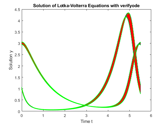
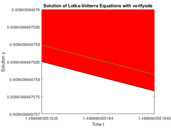
Zooming into the plot of y_2 at time t = 1.49 shows that the first ode45 approximation v with default options (blue line) is not contained in the verifyode enclosure (red tube), thus cannot be correct. Note that the solutions with initial conditions y0.inf and y0.sup for ode45 are only specific samples, and they should be within the inclusion computed by verifyode which contains the solution of the Lotka-Volterra equations for all initial conditions within y0.

axis([1.48 1.496  0.9 0.92]);                                          % Zoom into the plot for y_2 at t = 1.49.

Zooming closer into the plot shows that the ode45 approximation w computed with higher accuracy (green line) is indeed contained in the red tube.

axis([1.4899665551835 1.4899665551845  0.909409649757 0.90940964976]); % Zoom into the plot for y_2 at t = 1.489966555184.

Finally, we remark that awa cannot integrate this ODE up to tf = 5.5. The reason is that the initial condition box y0 = midrad([1;3],0.05) is quite large and the nonlinear Lotka-Voltera equations transform it through time to shapes with curved boundaries which are much overestimated by awa's convex polytopes enclosures.

Example III - The Lorenz system

Consider the Lorenz system

$\begin{array}{ccl} y'_1 &=& \sigma(y_2-y_1) \ , \\ y'_2 &=& (\rho-y(3))y(1)-y(2) \ , \\ y'_3 &=& y_1 y_2 - \beta y_3 \end{array}$

for

$\sigma = 10, \quad \rho = 28, \quad \beta = 8/3.$

It is implemented by

function dydt = lorenz(t,y,i)
  sigma = 10;
  rho = 28;
  if nargin == 2 || isempty(i) || i == 3
    if isfloat(y)
      beta = 8/3;
    else
      beta = iv2intval(iv_rdivide(8,3));
    end
  end
  if nargin == 2 || isempty(i)
    dydt = y;
    dydt(1) = sigma.*(y(2)-y(1));
    dydt(2) = (rho-y(3)).*y(1)-y(2);
    dydt(3) = y(1).*y(2)-beta.*y(3);
  else
    switch i
      case 1
        dydt = sigma.*(y(2)-y(1));
      case 2
        dydt = (rho-y(3)).*y(1)-y(2);
      case 3
        dydt = y(1).*y(2)-beta.*y(3);
    end
  end

The system shall be solved for interval initial conditions

$y_0 \in [-8.001,-7.998] \times [7.998,8.001] \times [26.998,27.001]$

and integration period [t0,tf] = [0 3], see [E], Chapter 5. The following program computes two verified solutions with verifyode. The first uses QR preconditioning, the second uses shrink wrapping. A third enclosure is computed with awa and evaluation method 4, see the demo of awa for details. All three enclosures are displayed for the final time point tf = 3. Furthermore, MATLAB's non-verified solver ode45 is used to compute an approximate solution of high accuracy where the midpoint of y0 is taken as initial condition.

t0 = 0;
tf = 3;
% verified enclosure of initial values
y0 = intval(' [-8.001,-7.998] [7.998,8.001] [26.998,27.001] ');
y0_mid = mid(y0);

format short infsup
progress(inf);  % Do not display a progress window.

disp('1. verifyode with QR preconditioning:')
options = verifyodeset('order',10, 'shrinkwrap',0, 'precondition',1, 'blunting',0,...
                       'h0',0.05, 'h_min',1e-3, 'loc_err_tol',1e-11, 'sparsity_tol',1e-20);
tic
[Tp,Yp,Yrp] = verifyode(@lorenz,[t0,tf],y0,options); % verifyode with QR preconditioning
run_time = toc
[~,yp_end] = verifyode_disp(Tp,Yp,Yrp,y0,tf);
disp(' ')
disp('2. verifyode with shrink wrapping')
options = verifyodeset('order',10, 'shrinkwrap',1, 'precondition',0, 'blunting',0,...
                       'h0',0.05, 'h_min',1e-3, 'loc_err_tol',1e-11, 'sparsity_tol',1e-20);
tic
[Ts,Ys] = verifyode(@lorenz,[t0,tf],y0,options);     % verifyode with shrink wrapping
run_time = toc
[~,ys_end] = verifyode_disp(Ts,Ys,[],y0,tf);
disp(' ')
disp('3. awa with evaluation method 4')
options = awaset('order',10, 'h0',0.1, 'h_min',1e-4, 'EvalMeth',4, 'AbsTol',1e-16, 'RelTol',1e-16);
tic
[t_awa,y_awa] = awa(@lorenz,@lorenz_jac,[t0,tf],y0,options);
run_time = toc
[~,y_awa_end] = awa_disp(t_awa,y_awa,[],tf);         % awa
disp(' ')
disp('4. ode45 with high accuracy')
options_ode45 = odeset('RelTol',1e-13, 'AbsTol',[1e-13 1e-13 1e-13]);
tic                                                  % ode45
[t_ode45,y_ode45] = ode45(@lorenz,[t0,tf],y0_mid,options_ode45);
run_time = toc
y_ode45_end = y_ode45(end,:)
disp(' ');
% Check whether the ode45 result is contained in the verifyode and awa enclosures.
incl = all(in(y_ode45_end,yp_end))  && ...
       all(in(y_ode45_end,ys_end))  && ...
       all(in(y_ode45_end,y_awa_end))

1. verifyode with QR preconditioning:
run_time =
   29.6355
t = 3
    [y_1] = [   -0.8241,   -0.7892]    d([y_1]) = 3.48e-02
    [y_2] = [   -0.2722,   -0.2274]    d([y_2]) = 4.47e-02
    [y_3] = [   19.2187,   19.2350]    d([y_3]) = 1.62e-02
 
 
2. verifyode with shrink wrapping
run_time =
   85.9618
t = 3
    [y_1] = [   -0.8303,   -0.7831]    d([y_1]) = 4.71e-02
    [y_2] = [   -0.2853,   -0.2146]    d([y_2]) = 7.06e-02
    [y_3] = [   19.1864,   19.2673]    d([y_3]) = 8.07e-02
 
 
3. awa with evaluation method 4
run_time =
   38.5207
t = 3
    [y_1] = [   -0.8352,   -0.7780]    d([y_1]) = 5.72e-02
    [y_2] = [   -0.2913,   -0.2084]    d([y_2]) = 8.28e-02
    [y_3] = [   19.1960,   19.2574]    d([y_3]) = 6.13e-02
 
 
4. ode45 with high accuracy
run_time =
    0.0695
y_ode45_end =
   -0.8066   -0.2499   19.2267
 
incl =
  logical
   1

The shortest runtime and the tightest enclosure is computed by verifyode with QR preconditioning. The enclosures of y_1 and y_2 computed with verifyode and shrink wrapping are better than those obtained with awa, whereas y_3 is better enclosed by awa.

The following program uses the function plottaylormodel_1d to plot enclosures that are overall verified, i.e., zooming in at any position always shows red verified lower and green verified upper bounds of the solution.

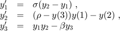
figure
title('Solution of Lorenz system with verifyode')
hold on
% The constants kmax1, kmax2, kmax3 are optional subdivision numbers for
% Taylor model domains, see the documentation of function plottaylormodel_1d.
kmax1 = 2;
kmax2 = 2;
kmax3 = 2;
plottaylormodel_1d(Ys(:,1),[],kmax1,kmax2,kmax3); % enclosure for y1
plottaylormodel_1d(Ys(:,2),[],kmax1,kmax2,kmax3); % enclosure for y2
plottaylormodel_1d(Ys(:,3),[],kmax1,kmax2,kmax3); % enclosure for y3
t = t_ode45;
y = y_ode45;
fig = plot(t,y(:,1),'k',t,y(:,2),'b',t,y(:,3),'c'); % approximate ode45 results
xlabel('Time t')
ylabel('Solution y')
legend(fig,'y_1','y_2','y_3')
hold off

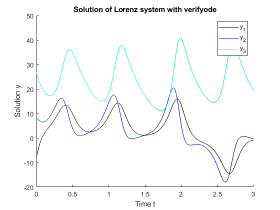
Zooming into the plot for y_2 (approximate solution by ode45 in blue) at t = 2.2 shows the verified lower and upper bounds plotted in red and green, respectively:

axis([2.11 2.25 -2.95 -2.45]);     % Zoom in on the plot for y_2 at t = 2.2.

If the enclosure obtained by verifyode with QR preconditioning shall be ploted in the same way, then left and right Taylor models Yp and Yrp must be concatenated first. This is done by the function tie. Suppose we only want to look at the second component y_2. Its left Taylor models are Yp(:,2) which must be concatenated with the right Taylor models Yrp:

Z = tie(Yp(:,2),Yrp);

The following program plots the Taylor model Z with red lower and green upper bound, and the awa enclosure as a yellow tube. Moreover, two new ode45 solutions are computed, one for initial condition y0.inf = [-8.001 , 7.998 , 26.998] (cyan dots) and one for initial condition y0.sup = [-7.998 , 8.001 , 27.001] (blue dots).

figure
plot(t_awa,y_awa(:,2),'y');     % awa enclosure (yellow tube)
hold on
title('Solution y_2 of Lorenz system')
xlabel('Time t')
ylabel('Solution y_2')
plottaylormodel_1d(Z,[],3,3,3); % verifyode enclosure for y2 (red and green lines)
[t_inf,y_inf] = ode45(@lorenz,Tp,y0.inf,options_ode45);
[t_sup,y_sup] = ode45(@lorenz,Tp,y0.sup,options_ode45); % ode45 for y0.sup
plot(t_inf,y_inf(:,2),'.c');    % ode45 result for y0.inf (cyan dots)
plot(t_inf,y_sup(:,2),'.b');    % ode45 result for y0.sup (blue dots)
axis([2.11 2.25 -2.92 -2.58]);  % Zoom in on the plot at t = 2.2.
hold off

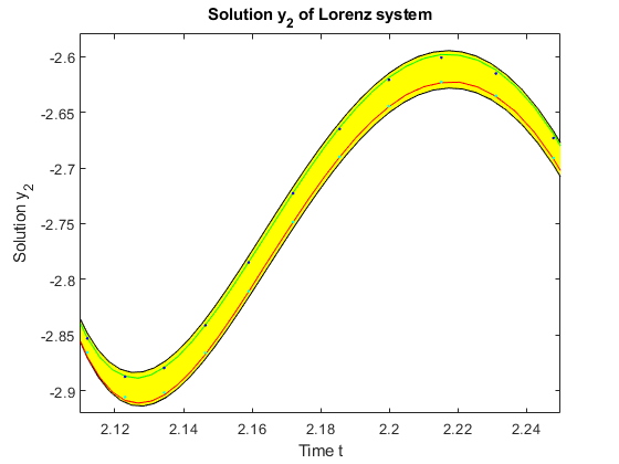
The approximate solutions by ode45 for initial conditions at the lower and the upper bounds of y0, respectively, suggest that the verified solution by awa is tight, and the verified solution by verifyode is almost as tight as possible.

Example IV - The van der Pol equation, a second order ODE

Consider the van der Pol equation

$$y'' - c (1-y^2)y'+y = 0 ,$$

where c > 0 is a scalar parameter, see Example II of the awa demo. Rewrite this equation as a system of first-order ODEs using the substitution y_1 := y and y_2 := y'. The resulting system is

$\begin{array}{ccl} y'_1 &=& y_2 \ , \\ y'_2 &=& c (1-y_1^2)y_2-y_1 \ . \end{array}$

The function file van_der_pol.m represents the van der Pol equation, using c = 1.

function dydt = van_der_pol(t,y,i)
  if nargin < 3 || isempty(i)
    dydt = [y(2) ; (1-sqr(y(1))).*y(2)-y(1)];
  else
    switch i
      case 1
        dydt = y(2);
      case 2
        dydt = (1-sqr(y(1))).*y(2)-y(1);
    end
  end

Solve the ODE on the time interval [0,10] with interval initial values y_0 = [2.999,3.001]x[-3.001,-2.999], see [E], Chapter 5. Three distinct option settings are used for three runs of verifyode:

shrink wrapping without blunting
shrink wrapping with blunting
QR preconditioning

y0 = midrad([3;-3],1e-3); % interval initial values
t0 = 0;
tf = 10;
tspan = [t0 tf];          % integration interval
order = 10;               % Taylor model order
h0 = 0.1;                 % initial step size
h_min = 0.005;            % minimum step size
l_tol = 1e-11;            % local error tolerance
s_tol = 1e-20;            % sparsity tolerance

disp('1. shrink wrapping without blunting:')
options = verifyodeset('order',order, 'shrinkwrap',1, 'precondition',0, 'blunting',0,...
                       'h0',h0, 'h_min',h_min, 'loc_err_tol',l_tol, 'sparsity_tol',s_tol);
tic
[Ts,Ys] = verifyode(@van_der_pol,tspan,y0,options);
run_time = toc
[ts,ys] = verifyode_disp(Ts,Ys,[],y0,tf);
disp(' ')
disp('2. shrink wrapping with blunting:')
options = verifyodeset('order',order, 'shrinkwrap',1, 'precondition',0, 'blunting',1, 'blunting factor',0.1,...
                       'h0',h0, 'h_min',h_min, 'loc_err_tol',l_tol, 'sparsity_tol',s_tol);
tic
[Tsb,Ysb] = verifyode(@van_der_pol,tspan,y0,options);
run_time = toc
[tsb,ysb] = verifyode_disp(Tsb,Ysb,[],y0,tf);
disp(' ')
disp('3. QR preconditioning:')
options = verifyodeset('order',order, 'shrinkwrap',0, 'precondition',1, 'blunting',0,...
                       'h0',h0, 'h_min',h_min, 'loc_err_tol',l_tol, 'sparsity_tol',s_tol);
tic
[Tp,Yp,Yrp] = verifyode(@van_der_pol,tspan,y0,options);
run_time = toc
[tp,yp] = verifyode_disp(Tp,Yp,Yrp,y0,tf);

1. shrink wrapping without blunting:
run_time =
   17.0901
t = 10
    [y_1] = [   -0.6325,   -0.5951]    d([y_1]) = 3.73e-02
    [y_2] = [   -2.6409,   -2.6272]    d([y_2]) = 1.36e-02
 
 
2. shrink wrapping with blunting:
run_time =
   28.1934
t = 10
    [y_1] = [   -0.6240,   -0.6034]    d([y_1]) = 2.05e-02
    [y_2] = [   -2.6383,   -2.6302]    d([y_2]) = 8.01e-03
 
 
3. QR preconditioning:
run_time =
    6.7679
t = 10
    [y_1] = [   -0.6230,   -0.6044]    d([y_1]) = 1.85e-02
    [y_2] = [   -2.6379,   -2.6306]    d([y_2]) = 7.22e-03

Method 3 (QR preconditioning) is the fastest with tightest enclosures. Method 2 (shrink wrapping with blunting) provides the second-best enclosures but is the slowest. Method 1 (shrink wrapping without blunting) gives the widest enclosures which shows that blunting of ill-conditioned matrices during shrink wrapping is advantageous for the van der Pol system. For other, better conditioned ODEs blunting may not have any effect.

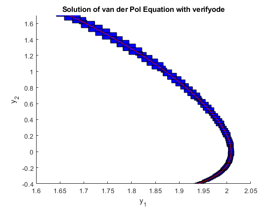
Finally, the result of method 1 is drawn as a verified phase portrait where y_2 is plotted against y_1. For comparison, the ODE is also solved with ode45 for initial conditions y0 = (3,-3) which is the midpoint of the interval initial conditions for verifyode.

figure
hold on
title('Solution of van der Pol Equation with verifyode');
xlabel('y_1');
ylabel('y_2');
tt = linspace(t0,tf,1e3);    % Create fine time grid for plotting.
plottaylormodel(Ys,tt,[],1); % Plot verfied phase portrait.
options_ode45 = odeset('RelTol',1e-12,'AbsTol',[1e-12 1e-12]);
[t,y] = ode45(@van_der_pol,tspan,mid(y0),options_ode45);
plot(y(:,1),y(:,2),'r');     % Plot ode45 result as red line.
hold off

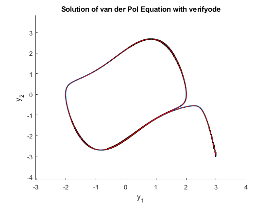
Zooming in on the plot at y1 = 1.8 and y2 = 0.6 shows that the ode45 result (red line) is quite centered in the verified plot (blue boxes).

axis([1.6 2.05 -0.4 1.7]);

Example V - A quadratic model problem

In [NJN1], Section 6.1, pages 257f, the simple quadratic second order problem u'' = u^2 is considered as a test case for QR preconditioning, see also [Bue3]. Rewritten as a two-dimensional first order system with y_1 := u and y_2 := u' this reads:

$\begin{array}{ccl} y'_1 &=& y_2 \ , \\ y'_2 &=& y_1^2 \ . \end{array}$

Interval initial values are taken as

$\begin{array}{ccl} y_0 &\in& (1\pm 0.05,-1\pm 0.05) \end{array}$

and integration is done for the time period [t0,tf] = [0,6]. The function file quadratic_problem.m implements the ODE:

function dydt = quadratic_problem(t,y,i)
  if nargin == 2 || isempty(i)
    dydt = [y(2) ; sqr(y(1))];
  else
    switch i
      case 1
        dydt = y(2);
      case 2
        dydt = sqr(y(1));
    end
  end

The following code uses Taylor models of order 18 and simple identity preconditioning to compute and display a verified enclosure at tf = 6. Afterwards, the function verifyode_phase_portrait is used to create two phase portraits.

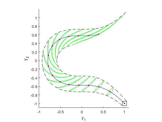
For each time point t_k = 0.4*k, k = 0,...,15 from the integration domain [t_0,t_f] = [0,6] the image of the polynomial part of the corresponding Taylor model is printed in green. Neglecting remainders this represents the enclosure of the ODE flow at that time point computed by the Taylor model method.

The blue solid line is the center trajectory, i.e., the solution for the point initial value (1,-1) which is the midpoint of the initial value box y_0. The red dots are the values of the center trajectory at the time points t_k. Finally, the black dashed lines are the trajectories originating at the lower left and upper right corners of y_0 . The plot shows that they almost exactly hit the endpoints of the elongated green shapes.

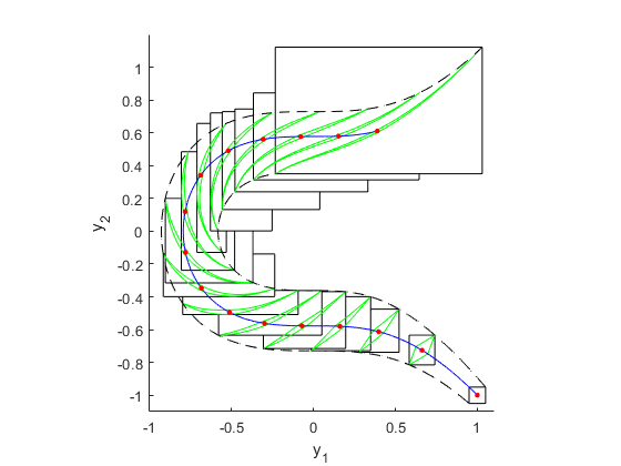
We want to state clearly that the plots described so far use non-verified floating point arithmetic and shall only give some impression of the ODE flow. Contrary to that, the black boxes in the second figure are overall verified enclosures of the ODE flow at the time points t_k. They tightly enclose the green shapes, demonstrating once again the sharpness of the Taylor model results. These boxes also show the advantage of the Taylor model approach. It allows to enclose sets with curved boundaries (green shapes) without much overestimation.

y0 = [1;-1]+infsup(-5,5)/100; % interval initial values [0.95,1.05]x[-1.05,-0.95]
t0 = 0;                       % definition of the time domain [t0,tf] = [0,6]
tf = 6;
odefun = @quadratic_problem;
options = verifyodeset('order',18,'precondition',-1,'h0',0.1,'h_min',0.01,'loc_err_tol',1E-11,'sparsity_tol',1E-20); % Identity preconditioning is used.
[T,Y,Yr] = verifyode(odefun,[t0,tf],y0',options);
disp(['Number of integration steps: ',num2str(length(T)-1)]);
verifyode_disp(T,Y,Yr,y0,tf,[],'longe');                       % Display verified enclosure at t = 6.
t = linspace(t0,tf,16);                                        % t = [0,0.4,0.8,1.2,...,6] contains the time points at which enclosing Taylor model ranges shall be visualized.
tt = linspace(t0,tf,1e3);                                      % fine time grid
[~,y_inf] = ode45(odefun,tt,y0.inf);                           % non-verified computation of the tractory originating at the lower left  corner of y0
[~,y_sup] = ode45(odefun,tt,y0.sup);                           % non-verified computation of the tractory originating at the upper right corner of y0
verifyode_phase_portrait(T,Y,Yr,y0,t);                         % first phase portrait with enclosing Taylor model ranges (green) at time points t(k) (red)
plot(y_inf(:,1),y_inf(:,2),'--k',y_sup(:,1),y_sup(:,2),'--k'); % Plot lower left and upper right corner trajectories.
axis([-1 1.1 -1.1 1.2])
hold on
verifyode_phase_portrait(T,Y,Yr,y0,t,[],[],1,1)                % second phase portrait which additionally contains (verified) box enclosures
plot(y_inf(:,1),y_inf(:,2),'--k',y_sup(:,1),y_sup(:,2),'--k'); % Plot lower left and upper right corner trajectories.
axis([-1 1.1 -1.1 1.2])
hold on

Number of integration steps: 31
t = 6
    [y_1] = [ -2.326433086661008e-001,  1.030204256727271e+000]    d([y_1]) = 1.26e+00
    [y_2] = [  3.497774700626797e-001,  1.122431220432956e+000]    d([y_2]) = 7.73e-01

Example VI - A Kepler problem for asteroid motion

In [H], p. 144ff, and [HBM] the motion of the asteroid 1997 XF11 is modeled by the Kepler problem

$\begin{array}{ccl} y'' &=& -\gamma y / (y_1^2+y_2^2+y_3^2)^{3/2} \ , \qquad \gamma = 0.9986 \ , \end{array}$

where y_1, y_2, y_3 are the (x,y,z)-coordinates of the asteroid in the solar system with the sun in its center, see also [E], p. 161ff. Rewritten as a six-dimensional first order ODE this reads

$\begin{array}{ccl} y_i' &=& y_{i+3} \ , \\ y'_{i+3} &=& -\gamma y_i/d, \quad i = 1,2,3 \ , \quad d = (y_1^2+y_2^2+y_3^2)^{3/2} \ . \end{array}$

The following interval initial values are considered:

$\begin{array}{cclc} y_1(0) &\in& -1.772 690 981 915 12 &\pm 0.5\cdot 10^{-7} \\ y_2(0) &\in& +0.148 721 485 234 295 5 &\pm 0.5\cdot 10^{-7} \\ y_3(0) &\in& -0.079 283 504 622 441 94 &\pm 0.5\cdot 10^{-7} \\ y_4(0) &\in& +0.237 203 191 651 623 7 &\pm 0.5\cdot 10^{-6} \\ y_5(0) &\in& +0.612 524 538 758 628 &\pm 0.5\cdot 10^{-6} \\ y_6(0) &\in& +0.045 832 175 721 656 24 &\pm 0.5\cdot 10^{-6} \end{array}$

Long term integration is done for 23 years. In scaled time units one year corresponds to $2\pi$ . Thus, the integration period is [t_0,t_f] = [0, $46\pi$ ]. An efficient implementation of the ODE may look as follows:

function dy = kepler(t,y,i)
  persistent g_
  if isempty(g_)
    g_ = intval(-9986)/1E4;                % verified inclusion of -0.9986
  end
  if nargin == 2 || isempty(i) || i >= 4
    if isfloat(y)                          % non-verified branch for MATLAB's non-verified ODE-solvers like ode45
      g = -0.9986;
    else                                   % verified branch for verifyode
      g = g_;
    end
    d = sqr(y(1)) + sqr(y(2)) + sqr(y(3));
    z = (d.^-1.5).*g;                      % Note that 1.5 is a floating-point number.
  end
  if nargin == 2 || isempty(i)
    dy = [y(4:6);y(1:3).*z];
  else
    if i <= 3
      dy = y(i+3);
    else
      dy = y(i-3).*z;
    end
  end

The following program uses blunted parallelepiped preconditioning. Parallelepiped preconditioning without blunting as well as curvilinear and identity preconditioning do not succeed integration for 23 years. QR preconditioning manages integration but gives significantly worse results than blunted parallelepiped preconditioning. Taylor model order 10 is chosen and a more sensitive relative $\varepsilon$ -inflation constant $\varepsilon_{rel}$ = 0.01 (1 percent) is used instead of the default value 0.1 (10 percent). This is done by setting the option eps_rel, see Section "Input Arguments".

WARNING: The expected runtime on a usual desktop PC is about four hours.

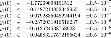
y0_mid = intval('-1.77269098191512 0.1487214852342955 -0.07928350462244194 0.2372031916516237 -0.612524538758628 0.04583217572165624');
r = [.5e-7;.5e-7;.5e-7;.5e-6;.5e-6;.5e-6];
y0 = y0_mid + infsup(-r,r); % interval initial values
t0 = 0;
tf = 46*intval('pi');       % tf = [tf.inf,tf.sup] is an interval enclosure of 46*pi.
tspan = [t0,tf.sup];        % integration period

% Execute verifyode with blunted parallelepiped preconditioning.
options = verifyodeset('order',10,'precondition',2,'blunting',1,'h0',0.1,'h_min',0.001,'loc_err_tol',1e-11,'sparsity_tol',1e-16,'eps_rel',0.01);
tic
[T,Y,Yr] = verifyode(@kepler,tspan,y0,options);
runtime = toc

disp(['Number of integration steps: ',num2str(length(T)-1)]);
verifyode_disp(T,Y,Yr,y0,tf,[],'longe'); % Display verified enclosure at t = 46*pi.

runtime =
   1.0169e+04
Number of integration steps: 1204
t = [  1.445132620651304e+002,  1.445132620651306e+002]
    [y_1] = [ -9.037458359243979e-001, -9.031675156232353e-001]    d([y_1]) = 5.78e-04
    [y_2] = [ -7.498342471077355e-001, -7.495871112032308e-001]    d([y_2]) = 2.47e-04
    [y_3] = [  8.639649869868784e-003,  8.676102355240028e-003]    d([y_3]) = 3.65e-05
    [y_4] = [  9.228458494872358e-001,  9.231946795210434e-001]    d([y_4]) = 3.49e-04
    [y_5] = [ -3.969999971194009e-001, -3.967100302479235e-001]    d([y_5]) = 2.90e-04
    [y_6] = [  6.026484211873011e-002,  6.026907478348357e-002]    d([y_6]) = 4.23e-06

Input Arguments

odefun : This is, as for all MATLAB ode-solvers like ode45, a function handle for the right-hand side f of the ODE y' = f(t,y). Different to MATLAB's ODE solvers, f must accept an additional, optional integer input argument i, that is:

dydt = odefun(t,y,i)

for a scalar t, a column vector y, and a positive integer i which is simply a function index between one and the dimension of the ODE system. If i is empty or if it is not passed to odefun, then odefun must return a column vector dydt that corresponds to f(t,y). If i is specified, then odefun shall only compute and return the i-th component f_i(t,y) of f(t,y). In case of a one-dimensional system there is no difference between calling odefun(t,y) and odefun(t,y,1).

We emphasize that odefun must accept all three input arguments, t, y, and i, even if some of the arguments are not used in the function. For example, to solve the one-dimensional system y' = 5y-3 use the function:

function dydt = odefun(t,y,i)
  dydt = 5.*y-3;

For a higher dimensional system, the output of odefun(t,y) is a vector. Each element in the vector is the solution to one equation. For example, to solve

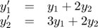
$\begin{array}{ccl} y'_1 &=& y_1 + 2y_2 \\ y'_2 &=& 3y_1 + 2y_2 \end{array}$

use the function:

function dydt = odefun(t,y,i)
  if nargin == 2 || isempty(i)
    dydt = y;                     % cheap initialization as column vector
    dydt(1) = y(1) + 2.*y(2);
    dydt(2) = 3.*y(1) + 2.*y(2);
  else
    switch i
      case 1
        dydt = y(1) + 2.*y(2);    % Compute only first component.
      case 2
        dydt = 3.*y(1) + 2.*y(2); % Compute only second component.
    end
  end

or alternatively:

function dydt = odefun(t,y,i)
  if nargin == 2 || isempty(i)
     dydt = [ y(1)+2.*y(2) ; 3.*y(1)+2.*y(2) ];
  else
    ...
  end

A function call odefun(t,y,1) only computes and returns the first equation dydt = y(1) + 2.*y(2). This possibility of equation-wise access to the ODE system allows to improve the performance of verifyode significantly.

The implementation of odefun may contain INTLAB interval operations and functions. Consider, for example, f(t,y) = cos( $\pi$ *y) + t. Then, since $\pi$ is not a floating-point number, odefun may be implemented rigorously as follows:

odefun = @(t,y,i) cos(intval('pi').*y) + t;

There is one special syntax rule that must be kept: If a constant value, either a floating-point number or an interval, shall be assigned to one of the components of dydt, then a typecasting using the function typeadjust must be done explicitly.

For example, the ODE y' = 1 must be implemented as

function dydt = odefun(t,y,i)
  dydt = typeadjust(1,y);

tspan = [t0,tf] specifies the integration interval. It must be a two element vector [t0,tf] where t0 is the starting time of integration and tf is the end time. Integration in negative direction, i.e., tf < t0 is supported. Note that t0 and tf must be floating-point numbers. In general this is no severe restriction and is either fulfilled anyway, or can easily be achieved by a shift and/or scaling of the time variable in the ODE function. This may lead to interval parameters in the ODE function.

MATLAB's ODE solvers like ode45 allow tspan = [t0,t1,t2,...,tf] to contain more than two elements, and in this case they return approximate values for the solution at these points. This is not allowed for verifyode. If verified enclosures of the solution at specific intermediate points [t1,t2,...] are sought, then this can be done a posteriori, see Example 1 and Section "Display results".

If a previous run of verifyode shall be resumed, then tspan must only contain the end time of the extended time domain which must be larger than that of the previous run (or smaller if integration was done in negative direction). For example, if a previous run of verifyode performed integration from t0 = 0 to tf = 3 by calling

  [T,Y,Yr] = verifyode(odefun,[0 3],y0,options);

then this run can be resumed to tf = 4 by calling

  [T_new,Y_new,Yr_new] = verifyode(odefun,4,{T,Y,Yr},options);

afterwards, whereby the input arguments odefun and options must remain unchanged. For the latter call tspan = 4 only contains the new end time, the starting time t0 = 3 is determined automatically from the input data {T,Y,Yr} which are the return arguments of the first call. Finally, the results T_new,Y_new,Yr_new of the second call contain the data for the whole extended time domain [0,4].

y0 : This is the initial value vector, i.e., y(t0) = y0, which may be a floating-point or interval vector.

If a previous run of verifyode shall be resumed, then y0 = {T,Y,Yr} must be a cell array containing the return arguments T,Y,Yr of the previous run, see the explanation for the input argument tspan.

options : option structure with components that are parameters of verifyode. The function verifyodeset can be used to create options similar to the MATLAB function odeset.

Example: options = verifyodeset('order',20, 'h0',1e-1, 'h_min',1e-3, 'loc_err_tol',1e-11);

This bounds the degree of Taylor models by 20, sets the initial and minimum step sizes (approximately) to 0.1 and 0.001, respectively, and limits the local error tolerance used for the automatic step size control to 1e-11.

The following options can be set:

order: bound of Taylor model degrees, see the first Section "Definition of Taylor models". The default is order = 12.
orders: individual degree bounds for the variables of the polynomial part of a Taylor model. The default is the empty set, meaning that no individual degree bounds are prescribed.
h0: initial step size. If h0 = 0 (default), then verifyode chooses the initial step size automatically. An experienced user may specify a reasonable nonzero value.
h_min: minimum step size. The default is h_min = 1e-4. Again, an experienced user may specify a reasonable nonzero value less than h0.
loc_err_tol: tolerance for the local error used in the automatic step size control. The default is loc_err_tol = 1e-10.
sparsity_tol: threshold amount for coefficients c of the polynomial part of a Taylor model. If |c| < sparsity_tol, then the coefficient is removed from the polynomial and the (small) error caused by this is transferred to the error interval of the Taylor model. See the first Section "Definition of Taylor models" for the definition of the polynomial part and the error interval of a Taylor model. The default is sparsity_tol = 1e-20.
shrinkwrap: flag for "shrink wrapping", 0: off (default), 1: on. See reference [Bue1] for details on shrink wrapping.
precondition: preconditioning of Taylor models,
- 0: off (default),
- 1: QR preconditioning,
- 2: parallelepiped preconditioning,
- 3: curvilinear preconditioning,
- -1: identity preconditioning.
In general there is no overall method for choosing the best preconditioning method for a specific ODE somehow automatically in advance. In practice a trial and error approach may quickly lead to a decission. However, QR preconditioning is a stable method with good performance that is well-suited for long-term integration. See references [MB1], [NJN1], [Bue2], and especially [Bue3] for details on preconditioning.
CL_depth: depth of curvilinear basis used for curvilinear preconditioning. The default is n/2 rounded upwards where n is the dimension of the ODE. See references [MB1] and [Bue3] for details on curvilinear preconditioning.
CL_reffun: optional function handle of user specified reference trajectory for curvilinear preconditioning. The default is CL_reffun = [] (empty).
blunting: blunting of ill-conditioned matrices during shrink wrapping or parallelepiped preconditioning, 0: off (default), 1: on. See references [MB1], [NJN2], and [Bue3] for details on blunting.
blunting factor: If blunting is switched on, then the so-called blunting factors are chosen as a factor e times the matrix column lengths. The factor e can be specified by this option. The default is e = 1e-3.
bounder: method for bounding the image of the polynomial part of a Taylor model,
- 'NAIVE': use interval arithmetic directly (default),
- 'LDB' : Linear Dominated Bounder, see references [M] and [N] for details on the LDB-method,
- 'BSB' : Bernstein Bounder, Bernstein polynomials are used as described by Titi and Garloff [TG].
eps_rel: relative epsilon inflation constant for inclusion step of Picard iteration. The default is eps_rel = 0.1, i.e., 10 percent. For proceeding more sensitively it can be advantageous to use a smaller value like eps_rel = 0.01, i.e., 1 percent.
eps_abs: absolute epsilon inflation constant for inclusion step of Picard iteration. The default is eps_abs = 2e-16.
Taylor expansion method: method for non-verified computation of the Taylor series of the ODE flow,
- 'Picard': Taylor expansion by Picard iteration (default),
- 'Lie' : Lie derivative method.
See reference [MB2] for details on the Lie derivative method. In our MATLAB implementatation the Lie derivative method turns out to be slower than the Picard iteration method. However, it might be interesting for the user to see how the Lie derivative method works.

Output Arguments

T: Array of time grid points with T(1) = t0 and T(m) = tf, where tspan = [t0,tf] is the integration interval, and m = length(T).
Y: Taylor model enclosure of the solution. Each row of the Taylor model array Y represents an inclusion of the solution y on a time interval of the time grid T. Precisely, for t in [T(j),T(j+1)] the solution y(t) at time t is contained in the set

$Y_j(t) = \{ (p_1(x,t)+e_1,\dots,p_n(x,t)+e_n)~|~ x \in [-1,1]^n, e_i \in E_i, i=1,\dots,n \}$

where n is the dimension of the ODE, p_i is the polynomial part and E_i is the error interval of the Taylor model Y(j,i), j = 1,..,m-1, i=1,...,n.

If preconditioning is switched on, see the description of the input argument "option", then Y only contains the so-called (time-dependent) left Taylor models. The corresponding (time-independent) right Taylor models are returned in the third output argument Yr.

Yr: For fixed time step j, the yl_i := Y(j,i), i = 1,...,n, are the left (time-dependent) Taylor models for t in [T(j),T(j+1)]. The corresponding (time-independent) right Taylor models are yr_i := Yr(j,i), i = 1,...,n. The ODE-flow on [T(j),T(j+1)] is given by the concatenation of left and right Taylor models:

$z_i(x,t) := yl_i(yr_1(x),...,yr_n(x),t) \quad $, $i=1,...,n,$

where $x = (x_1,...,x_n) \in [-1,1]^n$ are the spacelike variables. For technical reasons of postprocessing, left and right Taylor models are returned separately by verifyode if preconditioning is switched on. If preconditioning is switched off, then Yr is empty.

Display results

Call

[t,z] = verifyode_disp(T,Y,Yr,y0,tt);

to compute and display verified interval enclosures z of the solution y at arbitrarily chosen times tt in [t0,tf], see the examples. The input parameters T,Y,Yr are the output arguments of verifyode which can be directly passed to verifyode_disp. The fourth input argument y0 is the initial condition, and the fifth optional input argument tt is a floating-point or interval vector of time points or time intervals in [t0,tf] at which the enclosures shall be computed. If tt is not specified, then tt = T is taken by default.

The output argument t is tt returned as a column vector. If tt is a floating-point vector, then t is sorted in ascending order. Each row j of the interval array z corresponds to an enclosure of the solution at time t(j). (Recall that t(j) may be an interval.) This means that y_i(t(j)) is contained in z(j,i), j = 1,...,m, i = 1,...,n , where m = length(t) and n is the dimension of the ODE system. In other words, the column z(:,i) contains the enclosures of component y_i at all time points (or time intervals) t, i = 1,...,n. The call [t,z] = verifyode_disp(T,Y,Yr,y0,tt,false); suppresses formatted displaying the result.

References

[E]    I. Eble, Ueber Taylor-Modelle,
       Dissertation at Karlsruhe Institute of Technology, 2007 (written in German),
       Riot, C++-implementation, http://www.math.kit.edu/ianm1/~ingo.eble/de
[H]    J. Hoefkens, Rigorous numerical analysis with high-order Taylor models,
       Dissertation at Michigan State University, 2001
[HBM]  J. Hoefkens, M. Berz, K. Makino, Controlling the wrapping effect in the solution of ODEs for asteroids,
       Reliable Computing 8, pp. 21-41, 2003
[M]    K. Makino, Rigorous analysis of nonlinear motion in particle accelerators,
       Dissertation at Michigan State University, 1998
[MB1]  K. Makino and M. Berz, Suppression of the wrapping effect by Taylor model - based validated integrators,
       MSU HEP Report 40910, 2003
[MB2]  K. Makino and M. Berz, Rigorous Integration of flows and ODEs using Taylor models,
       Symbolic Numeric Computation 2009, pp. 79-84, 2009
[NJN1] M. Neher, K.R. Jackson, N.S. Nedialkov, On Taylor model based integration of ODEs,
       SIAM J. Numer. Anal. 45(1), pp. 236-262, 2007
[NJN2] M. Neher, K.R. Jackson, N.S. Nedialkov, On the blunting method in verified integration of ODEs,
       Reliable Computing 23, pp. 15-34, 2016
[N]    A. Neumaier, Taylor forms -- use and limits,
       Reliable Computing 9, pp. 43-79, 2003
[TG]   J.Titi, J. Garloff, Matrix methods for the tensorial Bernstein form,
       Applied Mathematics and Computation 346, pp. 254-271, 2019
[Bue1] F. Buenger, Shrink wrapping for Taylor models revisited,
       Numerical Algorithms 78(4), pp. 1001-1017, 2018
[Bue2] F. Buenger, A Taylor model toolbox for solving ODEs implemented in MATLAB/INTLAB,
       Journal of Computational and Applied Mathematics 368, Article 112511, 2020
[Bue3] F. Buenger, Preconditioning of Taylor models, implementation and test cases,
       submitted for publication 2020

Enjoy INTLAB

The Taylor model toolbox as well as this demo was written by Florian Buenger, Institute for Reliable Computing, Hamburg University of Technology.

INTLAB was designed and written by S.M. Rump, head of the Institute for Reliable Computing, Hamburg University of Technology. Suggestions are always welcome to rump (at) tuhh.de