DEMOSTDFCTS Interval standard functions in INTLAB

Contents

As explained in "DEMOINTVAL", standard functions with interval argument compute an inclusion of the true function value or the true function range.

Input arguments I

Special care is necessary if an input argument is not a floating-point number. For example,

format long _
x = intval([2.5 -0.3]);
y = erf(x)

intval y = 
   0.99959304798255  -0.32862675945912

computes the true range of the error function erf(2.5), but not necessarily of erf(-0.3). To obtain true results use

x = intval('2.5 -0.3');
y = erf(x)

intval y = 
   0.99959304798255
  -0.32862675945912

Note that intval converts a character string representing a vector always into a column vector. To see the accuracy of the result, the infsup-notation may be used:

infsup(y)
relerr(y)

intval y = 
[   0.99959304798255,   0.99959304798256] 
[  -0.32862675945913,  -0.32862675945912] 
ans =
   1.0e-15 *
   0.055533750803183
   0.422296341011770

Input arguments II

Similarly, the range of a function is included by

x = intval('[2.5,2.500001]')
y = erf(x)

intval x = 
   2.500001________
intval y = 
   0.99959305______

Note that the large diameter of the output is due to the large diameter of the input.

Accuracy of standard functions

The complementary error function erfc(x) is defined by 1-erf(x). It rapidly approximates 1 for larger x. In this case erfc(x) is much more accurate than 1-erf(x).

x = intval(5);
y1 = erfc(x)
y2 = 1 - erf(x)
infsup([y1;y2])

intval y1 = 
  1.0e-011 *
   0.15374597944280
intval y2 = 
  1.0e-011 *
   0.15375_________
intval  = 
  1.0e-011 *
[   0.15374597944280,   0.15374597944281] 
[   0.15374368445009,   0.15375478668034] 

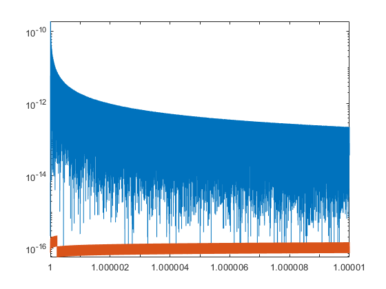
Sometimes the built-in standard functions are not very accurate:

x = linspace(1+1e-14,1+1e-5,100000);
y = acoth(x); Y = acoth(intval(x));
close, semilogy( x,abs((y-Y.mid)./(y+Y.mid)), x,relerr(Y) )

Nonlinear equations involving standard functions I

The zero of a nonlinear function may be approximated by some Newton procedure. Consider

x = linspace(0,10);
f = @(x) erf(x)-sin(x)
close
plot(x,f(x),x,0*x)

f =
  function_handle with value:
    @(x)erf(x)-sin(x)

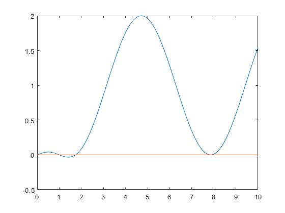
The graph shows the function erf(x)-sin(x) between 0 and 10. Besides the obvious root zero there seem to be two small roots near 1 and 2, and mathematically it follows that there must be two roots near 8.

To approximate the roots, a Newton procedure may be used. For example

x = 1;
for i=1:5
  y = f(gradientinit(x));
  x = x - y.x/y.dx
end

x =
   1.009823156064284
x =
   1.009829234350912
x =
   1.009829234354570
x =
   1.009829234354571
x =
   1.009829234354570

Inclusion of the solution of nonlinear systems with standard functions

As expected, the iteration converges very rapidly. The final value is a very good approximation of a root of f, and an inclusion is computed by

Y = verifynlss(f,x)

intval Y = 
   1.00982923435457

The range of a function and overestimation

The computed inclusion of the range of a function is a true estimate, but may be not sharp:

x = infsup(0,1);
yinf = f(x)

intval yinf = 
[  -0.84147098480790,   0.84270079294972] 

The inclusion can be improved using affine interval arithmetic:

yaff = f(affari(x))

affari yaff = 
[  -0.05999375863532,   0.10111067175095] 

Nonlinear equations involving standard functions II

More interesting is the root cluster near x=8. An attempt to compute inclusions fails:

Y1 = verifynlss(f,7.5)
Y2 = verifynlss(f,8.5)

intval Y1 = 
                NaN
intval Y2 = 
                NaN

The reason is that numerically this is a double zero because erf(8) is very close to 1, as can be checked by erfc(8) = 1-erf(8) :

y = erfc(intval(8))

intval y = 
  1.0e-028 *
   0.11224297172982

At least an inclusion of the extremum of f near 8 can be computed. Clearly it must be near to 2.5*pi.

Y = verifylocalmin(f,8)
y = 2.5*pi

intval Y = 
   7.85398163397448
y =
   7.853981633974483

For interval enthusiasts an inclusion of 2.5*pi can be computed as well. Note, however, that this is only close to the extremum.

y1 = 2.5*intval('pi')

intval y1 = 
   7.85398163397448

Verification of two roots

In the previous example, the function f has a nearly double root. It can be shown that a perturbed function g has a true double root:

Y = verifynlss2(f,8);
root = Y(1)
perturbation = Y(2)

intval root = 
   7.85398163397448
intval perturbation = 
  1.0e-015 *
   0.______________

That shows that the function g(x) := f(x)-e with e included in the computed perturbation has a double root contained in Y(1).

Accuracy of the gamma function I

Usually, Matlab standard functions produce very accurate approximations. For example,

x = pi
y = gamma(pi)
Y = gamma(intval('pi'))

x =
   3.141592653589793
y =
   2.288037795340032
intval Y = 
   2.28803779534003

Here Y is a true inclusion of the value of the gamma function at the transcendental number pi: X=intval('pi') is an inclusion of the mathematical pi, and the gamma function for an interval argument produces an inclusion of all values, in particular for the transcendental number pi.

Accuracy of the gamma function II

For negative arguments something strange happens in Matlab. Consider

x1 = -171.5;
x2 = -172.5;
y1 = gamma(x1)
y2 = gamma(x2)

y1 =
   Inf
y2 =
   Inf

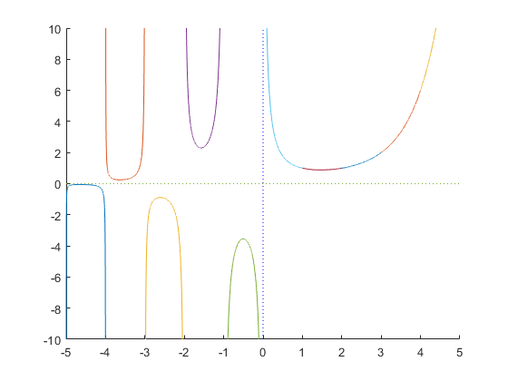
Regardless of the fact that for larger negative argument the gamma function is very small in absolute value, this cannot be true because the gamma function changes the sign when passing a negative integer:

 close
 axis([-5 5 -10 10])
 hold on
 for k=-5:5
   x = linspace(k,k+1,10000);
   plot(x,gamma(x))
 end
 plot([-5 5],[0 0],':',[0 0],[-10 10],'b:')
 hold off

The true values of the gamma function at x1=-171.5 and x2=-172.5 are indeed very small:

Y1 = gamma(intval(x1))
Y2 = gamma(intval(x2))

intval Y1 = 
  1.0e-309 *
   0.19316265431712
intval Y2 = 
  1.0e-311 *
  -0.1119783503283_

Accuracy of the gamma function III

In previous releases of Matlab, the accuracy of the gamma function near negative integers was very poor, sometimes with an error of 100 per cent. That was fixed from Matlab release 2018b on.

However, other problems with the gamma function remain. Consider

x = -171.25
y = gamma(x)
Y = gamma(intval(x))

x =
    -1.712500000000000e+02
y =
   Inf
intval Y = 
  1.0e-309 *
   0.98910291950447

Obviously gamma(x) must be very small in absolute value. In contrast, the Matlab result is infinity. Moreover,

x = -172.25
y = gamma(x)
Y = gamma(intval(x))

x =
    -1.722500000000000e+02
y =
   Inf
intval Y = 
  1.0e-311 *
  -0.5742252072588_

still produces +infinity in Matlab, whereas the sign must change from each integer interval to the next.

Inverse gamma function

Using automatic differentiation, values of the inverse gamma function are easily approximated. For example, compute x such that gamma(x)=3:

x = 4;
for i=1:5
    y = gamma(gradientinit(x)) - 3;
    x = x - y.x/y.dx
end

x =
   3.601948119538654
x =
   3.430611982891113
x =
   3.406291166087256
x =
   3.405870109547128
x =
   3.405869986309577

This value is approximate, the true value can be verified as follows:

X = verifynlss(@(x) gamma(x)-3 , 4)

intval X = 
   3.40586998630956

Minimum of the gamma function

Similarly, the minimum on the real axis of the gamma function is enclosed by

mu = verifylocalmin(@gamma,2)

intval mu = 
   1.46163214496836

Enjoy INTLAB

INTLAB was designed and written by S.M. Rump, head of the Institute for Reliable Computing, Hamburg University of Technology. Suggestions are always welcome to rump (at) tuhh.de

Published with MATLAB® R2020a