DEMOINTLAB_LARGER Some larger examples with INTLAB

Following are some larger examples using INTLAB, the Matlab toolbox for Reliable Computing. All computations are on my 3.0 GHz Laptop using Matlab R2020a under Windows.

Dense linear systems
Ill-conditioned dense linear systems
Sparse linear systems I
Sparse linear systems II
Larger least squares problems
Sparse least squares problems
Verified solution of a larger nonlinear system
An nonlinear optimization problem in 100 unknowns
An nonlinear optimization problem in 10,000 unknowns
Enjoy INTLAB

Dense linear systems

The following generates a dense linear system with n=5000 unknowns randomly with solution approximately all 1's. Since random matrices are generally well-conditioned, this is no real challenge concerning verification of the result.

Here and in the following we display the computing time for the Matlab built-in solver and for our verification routines. Note that this compares apples with oranges: the results of the verification routine are mathematically proved to be correct, including all rounding errors and the proof of non-singularity of the input matrix, whereas approximations are sometimes not correct, even without warning (see e.g. the section "Larger least squares problems").

Following the computing time for the Matlab solver A\b and for the verification INTLAB algorithm verifylss, some components of the solution as well as the minimum and median number of correct digits is displayed.

format short
n = 5000;
A = randn(n);
x = ones(n,1);
b = A*x;

tic
x = A\b;
disp(sprintf('Time for the built-in Matlab solver %5.1f [sec]',toc))

tic
X = verifylss(A,b);
disp(sprintf('Time for the verification algorithm %5.1f [sec]',toc))

v = [1:3 n-2:n];
format long
disp('Inclusion of the first and last three components')
X(v)
format short

r = relacc(X);
disp('Minimum and median number of correct digits')
[min(r) median(r)]

Time for the built-in Matlab solver   0.9 [sec]
Time for the verification algorithm   7.5 [sec]
Inclusion of the first and last three components
intval ans = 
   1.000000000000__
   1.00000000000___
   1.000000000000__
   1.000000000000__
   1.000000000000__
   1.000000000000__
Minimum and median number of correct digits
ans =
   12.1863   12.8860

Since the right hand side b is computed as A*x in floating-point, the true solution is approximately the vector of 1's, but not exactly. To force the solution to include the vector of 1's, the right hand side is computed as an inclusion of A*b. Such methods are often used as tests for verification algorithms.

bb = A*intval(ones(n,1));

tic
X = A\bb;
T = toc

v = [1:3 n-2:n];
format long
X(v)
format short

r = relacc(X);
disp('Minimum and median number of correct digits')
[min(r) median(r)]

T =
    8.9697
intval ans = 
   1.00000000______
   1.00000000______
   1.000000000_____
   1.00000000______
   1.00000000______
   1.00000000______
Minimum and median number of correct digits
ans =
    8.2149    8.9156

The computing time is roughly the same, but the inclusion is less accurate. However, the right hand side is now an interval vector, and the solution of all linear systems with a right hand side within bb is included.

For cond(A)~10^k, according to the well-known rule of thumb in numerical analysis, the accuracy of the inclusion should be roughly the number of correct digits in bb minus k. This is indeed true.

accX = median(r)
median(relacc(bb)) - log10(cond(A))

accX =
    8.9156
ans =
    9.0360

Ill-conditioned dense linear systems

Next an ill-conditioned linear system with n=5000 unknowns is generated with solution again roughly the vector of 1's. The condition number is approximately 10^14.

The computing time for the Matlab solver A\b and for the verification INTLAB algorithm verifylss, some components of the solution as well as the minimum and median number of correct digits is displayed.

The condition number implies that the accuracy of the inclusion should be roughly 16-14 = 2 correct digits. This indeed true.

format short
n = 5000;
A = randmat(n,1e14);
x = ones(n,1);
b = A*x;

tic
x = A\b;
disp(sprintf('Time for the built-in Matlab solver %5.1f [sec]',toc))

tic
X = verifylss(A,b);
disp(sprintf('Time for the verification algorithm %5.1f [sec]',toc))

v = [1:3 n-2:n];
format long _
disp('Approximation and inclusion of the first and last three components')
[x(v) X(v)]
format short

r = relacc(X);
disp('Minimum and median number of correct digits')
[min(r) median(r)]

disp('Median relative error of Matlab''s built-in solver')
median(relerr(x,X))

Warning: Matrix is close to singular or badly scaled. Results may be inaccurate.
RCOND =  7.060115e-17. 
Time for the built-in Matlab solver   0.9 [sec]
Time for the verification algorithm   9.7 [sec]
Approximation and inclusion of the first and last three components
intval ans = 
   1.00094688929043   1.000___________
   0.99494886444588   1.000___________
   1.00219981919006   1.00____________
   0.99182665162989   1.000___________
   0.99791283469176   1.000___________
   0.98800382446258   1.000___________
Minimum and median number of correct digits
ans =
    2.6427    4.1489
Median relative error of Matlab's built-in solver
ans =
    0.0024

Sparse linear systems I

By the principle of the used method, mainly symmetric positive definite matrices can be treated. The performance for general sparse matrices is not good; alas, basically no better method is known.

Consider for example matrix #356 from the Florida matrix market of dimension 52,329 with 2.6 million nonzero elements. The matrix looks as follows.

load('ct20stif')
A = Problem.A;
n = size(A,1)
b = A*ones(n,1);
close
spy(A)

n =
       52329

Example matrix #356 from the Florida matrix market of dimension 52,329 with 2.6 million nonzero elements

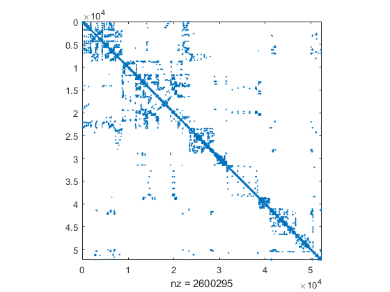
We display the timing the Matlab solver and the verification routine verifylss, and show the minimum and median accuracy of the inclusion. Note that the estimated condition number is 2e14.

CndEst = condest(A)

tic
x = A\b;
disp(sprintf('Time for the built-in Matlab solver %5.1f [sec]',toc))

tic
X = verifylss(A,b);
disp(sprintf('Time for the verification algorithm %5.1f [sec]',toc))

v = [1:3 n-2:n];
format long
disp('Inclusion of the first and last three components')
X(v)
format short

r = relacc(X);
disp('Minimum and median number of correct digits')
[min(r) median(r)]

CndEst =
   2.2282e+14
Time for the built-in Matlab solver   8.2 [sec]
Time for the verification algorithm  27.3 [sec]
Inclusion of the first and last three components
intval ans = 
   1.0000__________
   1.0000__________
   1.0000__________
   1.0000__________
   1.0000__________
   1.0000__________
Minimum and median number of correct digits
ans =
    1.3048    4.3151

Note that the verification algorithm requires about 50 per cent more computing time. For that, the result is mathematically verified to be correct.

Sparse linear systems II

Sometimes the verification routine is about as fast or even faster than the built-in Matlab solver. The next test matrix is #938 from the Florida matrix market. This matrix has dimension 36,000 with about 14 million nonzero elements.

load('nd12k')
A = Problem.A;
n = size(A,1)
b = A*ones(n,1);
close
spy(A)

n =
       36000

Test matrix #938 from the Florida matrix market

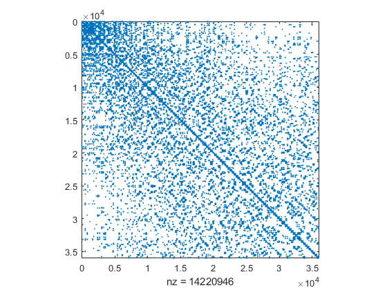
The estimated condition number is about 2.5e7. Now the verification routine is faster than the approximate solver.

CndEst = condest(A)

tic
x = A\b;
disp(sprintf('Time for the built-in Matlab solver %5.1f [sec]',toc))

tic
X = verifylss(A,b);
disp(sprintf('Time for the verification algorithm %5.1f [sec]',toc))

v = [1:3 n-2:n];
format long
disp('Inclusion of the first and last three components')
X(v)
format short

r = relacc(X);
disp('Minimum and median number of correct digits')
[min(r) median(r)]

CndEst =
   2.3458e+07
Time for the built-in Matlab solver  72.9 [sec]
Time for the verification algorithm  60.4 [sec]
Inclusion of the first and last three components
intval ans = 
   1.0000000_______
   1.0000000_______
   1.0000000_______
   1.0000000_______
   1.0000000_______
   1.0000000_______
Minimum and median number of correct digits
ans =
    7.4788    7.4788

The accuracy of the inclusion is as expected. We mention that verifylss applies by default an a priori minimum degree sorting. Usually this accelerates the method, but not always. For completeness we list the computing time of the approximate solver with this preordering.

tic
p = symamd(A);
x = A(p,p)\b(p);
disp(sprintf('Time for the built-in Matlab solver with preordering %5.1f [sec]',toc))

Time for the built-in Matlab solver with preordering  14.0 [sec]

Larger least squares problems

We first generate a dense 5000x500 matrix with condition number 1e12 to solve the corresponding least squares problem. The right hand side is the vector of 1's. The computing time of the built-in Matlab solver and the verification routine is displayed.

format short
m = 5000; n = 500;
A = randmat([m n],1e12);
b = ones(m,1);

tic
x = A\b;
disp(sprintf('Time for the built-in Matlab solver %5.1f [sec]',toc))

tic
X = verifylss(A,b);
disp(sprintf('Time for the verification algorithm %5.1f [sec]',toc))

Time for the built-in Matlab solver   0.2 [sec]
Time for the verification algorithm   1.9 [sec]

Next we show some components of the approximate solution computed x by Matlab and the verified inclusion X by INTLAB. From the accuracy of the verified inclusion, the accuracy of the Matlab approximation can be judged.

v = [1:3 n-2:n];
format long
disp('First and last three components: approximation and inclusion')
for i=v
  disp(sprintf('%17.7e %53s',x(i),infsup(X(i))))
  if i==3, disp([blanks(30) '...']), end
end
format short

r = relacc(X);
disp('Minimum and median number of correct digits')
[min(r) median(r)]

First and last three components: approximation and inclusion
    1.0919666e+12  [  1.092086454166138e+012,  1.092088921657310e+012] 
   -7.5627678e+10  [ -7.563294830245728e+010, -7.563266009874586e+010] 
    5.4424903e+10  [  5.443134775840061e+010,  5.443158296293536e+010] 
                              ...
    5.8657932e+10  [  5.867190775491055e+010,  5.867204906140201e+010] 
    1.5880300e+10  [  1.587581722935338e+010,  1.587594015730717e+010] 
    4.0533607e+10  [  4.053880768869635e+010,  4.053890131624199e+010] 
Minimum and median number of correct digits
ans =
    6.2511    7.1858

Sparse least squares problems

Following we display the timing and accuracy of the built-in Matlab routine and the verification routine verifylss for a larger least squares problem, namely matrix #2201. This is a problem with 37932 for 331 unknowns and about 137 thousand nonzero elements. The right hand side is again the vector of 1's.

load('abtaha2')
A = Problem.A;
[m n] = size(A)
b = ones(m,1);

tic
x = A\b;
disp(sprintf('Time for the built-in Matlab solver %5.1f [sec]',toc))

tic
X = verifylss(A,b);
disp(sprintf('Time for the verification algorithm %5.1f [sec]',toc))

v = [1:3 n-2:n];
format long
disp('Inclusion of the first and last three components')
X(v)
format short

r = relacc(X);
disp('Minimum and median number of correct digits')
[min(r) median(r)]

m =
       37932
n =
   331
Time for the built-in Matlab solver   0.3 [sec]
Time for the verification algorithm   1.3 [sec]
Inclusion of the first and last three components
intval ans = 
   0.86939173774958
   0.91891829446876
   0.93916745272555
  -0.99656428275776
  -0.79264335897383
   0.20386414427256
Minimum and median number of correct digits
ans =
   16.3189   16.9209

In this case we can judge from the inclusion that about 16 digits of the approximation are correct. With that information we ca judge that indeed the Matlab approximate solution is accurate to 13 digits as well.

Verified solution of a larger nonlinear system

The following example was proposed by Abbot and Brent and is implemented in the function test.

function y = test(x)
% Abbot/Brent     3 y" y + y'^2 = 0;    y(0)=0; y(1)=20;
% approximation   10*ones(n,1)
% solution        20*x^.75
  y = x;
  n = length(x); v=2:n-1;
  y(1) = 3*x(1)*(x(2)-2*x(1)) + x(2)*x(2)/4;
  y(v) = 3*x(v).*(x(v+1)-2*x(v)+x(v-1)) + (x(v+1)-x(v-1)).^2/4;
  y(n) = 3*x(n).*(20-2*x(n)+x(n-1)) + (20-x(n-1)).^2/4;

An inclusion of the solution for 5000 unknowns is computed. The timing, some components of the inclusion and the accuracy of the solution is displayed.

n = 5000;

tic
X = verifynlss(@test,10*ones(n,1));
disp(sprintf('Time for the verification algorithm %5.1f [sec]',toc))

v = [1:3 n-2:n];
format long
disp('Inclusion of the first and last three components')
X(v)
format short

r = relacc(X);
disp('Minimum and median number of correct digits')
[min(r) median(r)]

Time for the verification algorithm   3.9 [sec]
Inclusion of the first and last three components
intval ans = 
   0.03106851969020
   0.05424460056172
   0.07452016877319
  19.99100091446536
  19.99400075965309
  19.99700045481880
Minimum and median number of correct digits
ans =
   16.0514   16.6535

An nonlinear optimization problem in 100 unknowns

Consider the problem "bdqrtic" in

  Source: Problem 61 in
     A.R. Conn, N.I.M. Gould, M. Lescrenier and Ph.L. Toint,
     "Performance of a multifrontal scheme for partially separable optimization",
      Report 88/4, Dept of Mathematics, FUNDP (Namur, B), 1988.
      Copyright (C) 2001 Princeton University
      All Rights Reserved
  see bottom of file test_h.m

The model problem is

   N = length(x);      % model problem: initial approximation x=ones(N,1);
   I = 1:N-4;
   y = sum( (-4*x(I)+3.0).^2 ) + sum( ( x(I).^2 + 2*x(I+1).^2 + ...
             3*x(I+2).^2 + 4*x(I+3).^2 + 5*x(N).^2 ).^2 );

This function is evaluated by

   index = 2;
   y = test_h(x,index);

We first solve the corresponding nonlinear system in only 100 unknowns to compare with Matlab's built-in fminsearch.

n = 100;
index = 2;

disp('Floating-point approximation by fminsearch with restart')
optimset.Display='off';
x = ones(n,1);
tic
for i=1:5
  x = fminsearch(@(x)test_h(x,index),x,optimset);
  y = test_h(x,index);
  disp(sprintf('iteration %1d and current minimal value %7.1f',i,y))
end
disp(sprintf('Time for fminsearch with 5 restarts %5.1f [sec]',toc))
disp(' ')

xs = ones(n,1);
tic
X = verifylocalmin('test_h',xs,[],0,index);
disp(sprintf('Time for the verification algorithm %5.1f [sec]',toc))
Y = test_h(X,index);
disp(sprintf('Minimal value for stationary point %7.1f',Y.mid))

r = relacc(X);
disp('Minimum and median number of correct digits of stationary point')
[min(r) median(r)]

Floating-point approximation by fminsearch with restart
iteration 1 and current minimal value  6733.3
iteration 2 and current minimal value  2529.4
iteration 3 and current minimal value   587.9
iteration 4 and current minimal value   406.9
iteration 5 and current minimal value   378.9
Time for fminsearch with 5 restarts   3.4 [sec]
 
Time for the verification algorithm   0.1 [sec]
Minimal value for stationary point   378.8
Minimum and median number of correct digits of stationary point
ans =
   15.8753   15.8753

Only after 5 restarts, the approximation by fminsearch is of reasonable accuracy. However, that we know only by the verification method. The built-in Matlab routine fminsearch uses the Nelder-Mead algorithm without derivative, thus it is slow even for few unknowns.

An nonlinear optimization problem in 10,000 unknowns

Next we solve the previous nonlinear system in 10,000 unknowns with verification. The given starting vector is again x = ones(n,1). Note that during the computation x will be a vector of Hessians, each carrying a Hessian matrix, in total 10000^3 = 1e12 elements or 8 TeraByte - if not stored sparse.

n = 10000;
index = 2;
tic
X = verifylocalmin('test_h',ones(n,1),[],0,index);
disp(sprintf('Time for the verification algorithm %5.1f [sec]',toc))

r = relacc(X);
disp('Minimum and median number of correct digits')
[min(r) median(r)]

Time for the verification algorithm  34.1 [sec]
Minimum and median number of correct digits
ans =
   15.8084   15.8753

Notice the high accuracy of the result. Mathematically, the interval vector X is proved to contain not only a stationary point, but a true (local) minimum.

The proof for positive definiteness is included in the verification routine verifylocalmin. That proof may be performed separately as follows.

tic
y = test_h(hessianinit(X),index);
isLocalMinimum = isspd(y.hx)
disp(sprintf('Time for the verification algorithm %5.1f [sec]',toc))

isLocalMinimum =
  logical
   1
Time for the verification algorithm   0.2 [sec]

The latter command verified that the Hessian at all points in X is s.p.d., among them at the stationary point xx.

Enjoy INTLAB

INTLAB was designed and written by S.M. Rump, head of the Institute for Reliable Computing, Hamburg University of Technology. Suggestions are always welcome to rump (at) tuhh.de