DEMOGRADIENT Short demonstration of gradients

Contents

Some sample applications of the gradient toolbox

The gradient toolbox implements automatic differentiation in forward mode.

Initialization of gradients

In order to use automatic differentiation, the independent variables need to be identified and values have to be assigned. This is performed by the function "gradientinit". For example

format compact short _
u = gradientinit([ -3.1 ; 4e-3 ])

gradient value u.x = 
   -3.1000
    0.0040
gradient derivative(s) u.dx = 
     1     0
     0     1

The total size of the input is the number of independent variables, in the example 2, hence u represents a column vector of length 2 and defines two independent variables u(1) and u(2) with gradients [1 0] and [0 1], respectively.

Operations between gradients

If at least one operand is of type gradient, operations are executed as gradient operations. For example,

x = gradientinit(3.5);
y = exp(3*x-sqrt(x))

gradient value y.x = 
   5.5924e+03
gradient derivative(s) y.dx = 
   1.5283e+04

For f(x):=exp(3*x-sqrt(x)), the result y contains in y.x the function value f(3.5) and in y.dx the derivative f'(3.5):

y.x, y.dx

ans =
   5.5924e+03
ans =
   1.5283e+04

Complex arguments

When evaluating the expression for another argument, use the same statement as before with new values.

x = gradientinit(-3.5+.2i);
y = exp(3*x-sqrt(x))

gradient value y.x = 
   7.6944e-06 - 2.4944e-05i
gradient derivative(s) y.dx = 
   2.9683e-05 - 7.2588e-05i

Access to the gradient

The principle works for functions in several unknowns the same way. Define, for example, the following function from R^3->R^3 :

f = @(x)( [ -2*x(1)*x(2)+4*x(3)^2 ; sin(x(2))/sqrt(pi-x(1)) ; atan(x(2)-x(3)) ] )
f([1.5;-1;0.7])

f =
  function_handle with value:
    @(x)([-2*x(1)*x(2)+4*x(3)^2;sin(x(2))/sqrt(pi-x(1));atan(x(2)-x(3))])
ans =
    4.9600
   -0.6568
   -1.0391

then the function value and gradient at [1.5;-1;0.7] is computed by

y = f(gradientinit([1.5;-1;0.7]))

gradient value y.x = 
    4.9600
   -0.6568
   -1.0391
gradient derivative(s) y.dx = 
    2.0000   -3.0000    5.6000
   -0.2000    0.4217         0
         0    0.2571   -0.2571

where y.x contains the function value and y.dx the gradient, which is in this case the Jacobian. The gradient with respect the third unknown x(3), for example, can be accessed by

y.dx(3,:)

ans =
         0    0.2571   -0.2571

However, it is recommended to use

y(3).dx

ans =
         0    0.2571   -0.2571

that is not to access the components of the gradient (Jacobian) but the gradient of the component. The advantage is visible when redefining the input function as a row vector:

f = @(x)( [ -2*x(1)*x(2)+4*x(3)^2  sin(x(2))/sqrt(pi-x(1))  atan(x(2)-x(3)) ] )
f([1.5;-1;0.7])

f =
  function_handle with value:
    @(x)([-2*x(1)*x(2)+4*x(3)^2,sin(x(2))/sqrt(pi-x(1)),atan(x(2)-x(3))])
ans =
    4.9600   -0.6568   -1.0391

Then the "Jacobian" is a three-dimensional array because the gradient is always stored in the "next" dimension:

y = f(gradientinit([1.5;-1;0.7]))

gradient value y.x = 
    4.9600   -0.6568   -1.0391
gradient derivative(s) y.dx(1,1,:) = 
    2.0000   -3.0000    5.6000
gradient derivative(s) y.dx(1,2,:) = 
   -0.2000    0.4217         0
gradient derivative(s) y.dx(1,3,:) = 
         0    0.2571   -0.2571

It is problematic to access the components of y.dx, while accessing the gradient of the component works as expected:

y(3).dx

ans =
         0    0.2571   -0.2571

The inverse Gamma function

We may want to calculate the inverse Gamma function using INTLAB's verified Gamma function. For example, compute u such that gamma(u) = 100. Consider the following simple Newton procedure with starting value u=5.

format long
u = gradientinit(5);
uold = u;
k = 0;
while abs(u.x-uold.x) > 1e-12*abs(u.x) | k < 1
  uold = u;
  k = k+1;
  y = gamma(u) - 100;
  u = u - y.x/y.dx;
end
k
u.x
gamma(u.x)

k =
     9
ans =
   5.892518696343773
ans =
   100

The inverse Gamma function with complex arguments

Neither Matlab nor INTLAB provide the Gamma function for complex arguments. However, we may use an approximation by Stirling's formula. For u -> inf,

                       1      1       139        571
 Gamma(u) ~ C * ( 1 + --- + ----- - ------- - --------- + ... )
                      12u       2         3           4
                            288u    51840u    2488320u

with

      -u  u-0.5
 C = e   u      sqrt(2*pi) .

The following function evaluates Stirling's formula. It is also suited for vector input.

function y = g(u)
    C = exp(-u) .* ( u.^(u-0.5) ) * sqrt(2.0*pi) ;
    v = (((( -571.0/2488320.0 ./ u - 139.0/51840.0 ) ./ u ...
         + 1.0/288.0) ./ u ) + 1.0/12.0 ) ./ u + 1.0;
    y = C .* v;

A corresponding inline function is

format long e
g = @(u) ( ( exp(-u) .* ( u.^(u-0.5) ) * sqrt(2.0*pi) ) .* ...
           ( (((( -571.0/2488320.0 ./ u - 139.0/51840.0 ) ./ u ...
             + 1.0/288.0) ./ u ) + 1.0/12.0 ) ./ u + 1.0 ) )
u = [ 3.5 61 5 ]
g(u)
gamma(intval(u))

g =
  function_handle with value:
    @(u)((exp(-u).*(u.^(u-0.5))*sqrt(2.0*pi)).*(((((-571.0/2488320.0./u-139.0/51840.0)./u+1.0/288.0)./u)+1.0/12.0)./u+1.0))
u =
     3.500000000000000e+00     6.100000000000000e+01     5.000000000000000e+00
ans =
     3.323346278704310e+00     8.320987112733666e+81     2.399999414518977e+01
intval ans = 
  3.32335097044784_e+000  8.32098711274139_e+081  2.400000000000000e+001

Note however that the approximation by Stirling's formula is of limited accuracy. The last line, a verified inclusion by INTLAB's Gamma function, indicates about 6 to 11 correct figures, depending on the magnitude of the argument.

Using Stirling's formula we may search u with g(u) = 100 + 100i. We use the same starting value u=5.

 u = gradientinit(5);
 uold = u;
 k = 0;
 while abs(u.x-uold.x) > 1e-12*abs(u.x) | k < 1
  uold = u;
  k = k+1;
  y = g(u) - 100 - 100i;
  u = u - y.x/y.dx;
 end
 k
 u.x
 g(u.x)

k =
    10
ans =
      6.701615293582063e+00 + 3.757828161591650e+00i
ans =
      1.000000000000003e+02 + 1.000000000000002e+02i

Due to approximation error in Stirling's formula, about six figures are correct.

Automatic differentiation with several unknowns

Automatic differentiation with several unknowns works the same way. Consider the following example by Broyden:

                             .5*sin(x1*x2) - x2/(4*pi) - x1/2  =  0
(1-1/(4*pi))*(exp(2*x1)-exp(1)) + exp(1)*x2/pi - 2*exp(1)*x1 )  =  0

with initial approximation [ .6 ; 3 ] and one solution [ .5 ; pi ]. The following inline function evaluates Broyden's function.

f = @(x) ( [ .5*sin(x(1)*x(2)) - x(2)/(4*pi) - x(1)/2 ; ...
             (1-1/(4*pi))*(exp(2*x(1))-exp(1)) + exp(1)*x(2)/pi - 2*exp(1)*x(1) ] )

f =
  function_handle with value:
    @(x)([.5*sin(x(1)*x(2))-x(2)/(4*pi)-x(1)/2;(1-1/(4*pi))*(exp(2*x(1))-exp(1))+exp(1)*x(2)/pi-2*exp(1)*x(1)])

Solution of a nonlinear system

The nonlinear system defined by Broyden's function is solved by Newton's procedure as follows:

 x = gradientinit([ .6 ; 3 ]);
 for i=1:5
  y = f(x);
  x = x - y.dx\y.x;
 end
 x

gradient value x.x = 
     4.999999999999999e-01
     3.141592653589794e+00
gradient derivative(s) x.dx = 
     1     0
     0     1

For simplicity, we omitted the stopping criterion (see above). Here, y.dx is the Jacobian, y.x the function value at x.x, and -y.dx\y.x is the correction obtained by the (approximate) solution of a linear system.

Verified solution of the nonlinear system

For verified solution of the nonlinear system, we need a correct definition of the function. The main point is to make sure that a function evaluation with interval argument computes an inclusion of the function value. So first the transcendental number pi has to be replaced by an interval containing pi:

cPi = intval('pi')

intval cPi = 
  3.141592653589794e+000

Second, Broyden's function contains exp(1), which would be computed in pure floating-point without extra care. This can be cured using exp(intval(1)).

However, a new problem arises. When replacing "pi" in the function by "cPi" and 1 by intval(1), the function is always evaluated in interval arithmetic; a pure floating point iteration is no longer possible.

To solve this problem, we have to know the type of the incoming unknown "x". If "x" is double, replace "cPi" and intval(1) by its midpoint, if "x" is an interval, use "cPi" and intval(1) as is. This is done as follows.

function  y = f(x)
  y = x;
  c1 = typeadj( 1 , typeof(x) );
  cpi = typeadj( midrad(3.14159265358979323,1e-16) , typeof(x) );
  y(1) = .5*sin(x(1)*x(2)) - x(2)/(4*cpi) - x(1)/2;
  y(2) = (1-1/(4*cpi))*(exp(2*x(1))-exp(c1)) + exp(c1)*x(2)/cpi - 2*exp(c1)*x(1);

This code is implemented in the function Broyden.m .

Real and interval function evaluation

Consider the following two function evaluations. First, f(x) is evaluated for real argument:

x = [ .6 ; 3 ];
Broyden(x)

ans =
    -5.180859919874536e-02
    -1.122276766667780e-01

Second, f(x) is evaluated with interval argument:

format _
x = [intval('.6') ; 3 ]
y = Broyden(x)

intval x = 
  6.00000000000000_e-001
  3.000000000000000e+000
intval y = 
 -5.1808599198745__e-002
 -1.1222767666678__e-001

The mathematical statement is the following. First, x is an interval vector such that x(1) is an inclusion of 0.6 and x(2)=3. Second, cPi is an interval containing the transcendental number pi. Third, y is an interval vector containing the exact value of Broyden's function evaluated at [ .6 ; 3 ].

Gradient function evaluation using ordinary intervals

Finally, we may define the interval x to be of type gradient:

x = gradientinit([intval('.6') ; 3 ])
Y = Broyden(x)

intval gradient value x.x = 
  6.00000000000000_e-001
  3.000000000000000e+000
intval gradient derivative(s) x.dx = 
  1.000000000000000e+000   0.000000000000000e+00
   0.000000000000000e+00  1.000000000000000e+000
intval gradient value Y.x = 
 -5.1808599198745__e-002
 -1.1222767666678__e-001
intval gradient derivative(s) Y.dx = 
 -8.40803142039631_e-001 -1.47738099953874_e-001
  6.7525716865843__e-001  8.65255979432265_e-001

The mathematical statement is that Y is an interval vector such that Y.x contains the exact value of Broyden's function evaluated at [ .6 ; 3 ], and Y.dx is an interval matrix containing the Jacobian of Broyden's function evaluated at [ .6 ; 3 ].

Gradient function evaluation using affine intervals

We may use affine arithmetic in gradient evaluations as well, for details see the affari demo:

x = gradientinit([affari(.6) ; 3 ])
Y = Broyden(x)

affari gradient value x.x = 
  6.000000000000000e-001
  3.000000000000000e+000
affari gradient derivative(s) x.dx = 
  1.000000000000000e+000   0.000000000000000e+00
   0.000000000000000e+00  1.000000000000000e+000
affari gradient value Y.x = 
 -5.1808599198745__e-002
 -1.1222767666678__e-001
affari gradient derivative(s) Y.dx = 
 -8.40803142039630_e-001 -1.47738099953874_e-001
  6.7525716865843__e-001  8.65255979432265_e-001

Verified solution of the nonlinear system with Broyden's function

The nonlinear system with Broyden's function and the given starting value [ .6 ; 3 ] can be solved with verification by

Y = verifynlss(@Broyden,[ .6 ; 3 ])

intval Y = 
  5.00000000000000_e-001
  3.14159265358979_e+000

The first parameter gives the name of the function such that Broyden(x) evaluates the function at "x". The result vector Y is verified to contain a real vector xhat such that f(xhat)=0. This solution X of the nonlinear system is proved to be unique within Y. This statement is mathematically true, it is taken care of all procedural, approximation and rounding errors.

It follows that an inclusion is not possible if roots are very close together or multiple: Since uniqueness of the root is proved, an inclusion is only possible if roots can be separated. An escape of that is described in DEMOSLOPE.

All roots of Broyden's function

The root [ 0.5 ; pi ] is mentioned in the literature, however, there are many more roots. For example, there are seven roots in the box [-10,10]^2

format short
L = verifynlssall(@Broyden,infsup(-10,10)*ones(2,1))

intval L = 
   -0.2606    0.2994    0.5000    1.2943    1.3374    1.4339    1.4813
    0.6225    2.8369    3.1415   -3.1372   -4.1404   -6.8207   -8.3836

For more details, please visit the demo on global routines by demo toolbox intlab .

Verified solution of a nonlinear system with sparse gradients

Up to now we considered only toy examples to explain how the nonlinear system solver works. For a larger example consider the following example proposed by Abbot and Brent, which is implemented in the function test.

function y = test(x);
% Abbot/Brent     3 y" y + y'^2 = 0;    y(0)=0; y(1)=20;
% approximation   10*ones(n,1)
% solution        20*x^.75
  y = x;
  n = length(x); v=2:n-1;
  y(1) = 3*x(1)*(x(2)-2*x(1)) + x(2)*x(2)/4;
  y(v) = 3*x(v).*(x(v+1)-2*x(v)+x(v-1)) + (x(v+1)-x(v-1)).^2/4;
  y(n) = 3*x(n).*(20-2*x(n)+x(n-1)) + (20-x(n-1)).^2/4;

An inclusion of the solution for 1000 unknowns is computed by

format short
sparsegradient(50)
n = 1000;
tic
x = verifynlss(@test,10*ones(n,1));
toc
max(relerr(x))

===> Gradient derivative stored sparse for 50 and more unknowns
ans =
    50
Elapsed time is 0.284325 seconds.
ans =
   3.8277e-16

Verified solution of a nonlinear system with full gradients

Here we specified that gradients with 50 unknowns and more are stored in sparse mode. This is the default when calling "sparsegradient".

Forcing gradients to use full storage results in a significantly increase of computing time.

sparsegradient(inf)
n = 1000;
tic
x = verifynlss(@test,10*ones(n,1));
toc
max(relerr(x))

===> Gradient derivative always stored full
ans =
   Inf
Elapsed time is 1.284535 seconds.
ans =
   3.8277e-16

Verified solution of a nonlinear system with 10,000 unknowns

Note that the inclusion is of high accuracy. The results for a larger nonlinear system with 10,000 unknowns is as follows.

sparsegradient(0)
n = 10000;
tic
x = verifynlss(@test,10*ones(n,1));
toc
max(relerr(x))

===> Gradient derivative always stored sparse
ans =
     0
Elapsed time is 16.224590 seconds.
ans =
   5.3780e-16

Non-differentiable functions

The given function need not be differentiable everywhere. Consider, for example,

f = inline('abs(x)')
f(gradientinit(infsup(-.1,2)))

f =
     Inline function:
     f(x) = abs(x)
intval gradient value ans.x = 
[    0.0000,    2.0000] 
intval gradient derivative(s) ans.dx = 
  (1,1)             [   -1.0000,    1.0000] 

Verified solution of non-differentiable functions

The inclusion of a root is searched for near the given approximation. Consider

f = vectorize(inline('x*sinh(x)-3*exp(abs(x)-.5)+x*cos(x+1)+2*cosh(x)'))
close
x=linspace(-1,2.3);
plot(x,f(x),x,0*x)

f =
     Inline function:
     f(x) = x.*sinh(x)-3.*exp(abs(x)-.5)+x.*cos(x+1)+2.*cosh(x)

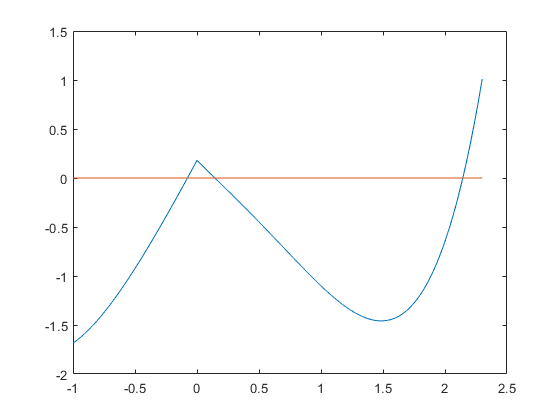
It seems there are three roots. Indeed,

format long
verifynlss(f,-.5)
verifynlss(f,.5)
verifynlss(f,2)

intval ans = 
  -0.07707181827987
intval ans = 
   0.14381565238483
intval ans = 
   2.14372206306996

there are three roots, and the inclusions are of high accuracy. One can also calculate an inclusion of multiple roots. Since the problem is ill-posed, it has to be regularized. Consider

X = verifynlss2(@(x)(sin(x)-1),1.5)

intval X = 
   1.57079632679489
  -0.00000000000000

It is proved that there exists some parameter e in X(2) such that the function g(x):=f(x)-e has a truly double root in X(1). Note the accuracy of the inclusions. It looks like the inclusion of e is a true zero. However, this is due to the "_"-format: add +/-1 to the last visible digit produces a valid inclusion:

format long e infsup
X

intval X = 
[  1.570796326794895e+000,  1.570796326794897e+000] 
[ -1.110223024625157e-016,  2.465190328815663e-032] 

The function "verifynlss2" is applicable to multivariate functions as well. For more details, see "help verifynlss" or "help verifynlss2" or

S.M. Rump: Verification methods: Rigorous results using floating-point arithmetic.
  Acta Numerica, 19:287-449, 2010.

to be downloaded from www.tuhh.de/ti3/rump/ and the literature cited over there.

Enjoy INTLAB

INTLAB was designed and written by S.M. Rump, head of the Institute for Reliable Computing, Hamburg University of Technology. Suggestions are always welcome to rump (at) tuhh.de

Published with MATLAB® R2020a