DEMOGLOBAL Global minima, constraint global minima and all roots

This is a short demonstration of INTLAB functions for global problems, in particular

The algorithms are based on

S.M. Rump. Mathematically Rigorous Global Optimization in Floating-Point Arithmetic. to appear in Optimization Methods & Software, 33(4-6):771-798, 2018.

Contents

Finding all roots of a univariate function within a box

Given a function f:R^n->R^n, algorithm "verifynlssall" finds all roots of f within a given box X. Let's start with a univariate function

format compact long _
close all
setround(0)                           % set rounding to nearest

f = @(x)(sin(x)+cos(x/2)+x/5)
x = linspace(-20,15);
plot(x,f(x),x,0*x)
title('sin(x)+cos(x/2)+x/5  in  [-20,15]')

f =
  function_handle with value:
    @(x)(sin(x)+cos(x/2)+x/5)

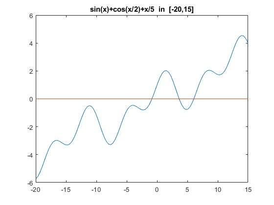
The graph suggests that f has three real roots near -1, 4 and 6, respectively. All real roots of f can be included as follows:

tic
X = infsup(-inf,inf);
[L,Ls] = verifynlssall(f,X)
toc

intval L = 
  -0.84041617394821   3.64287443341707   6.06278265338672
Ls =
     []
Elapsed time is 0.174157 seconds.

Here the columns of L are inclusions of roots of f, whereas Ls collects possible additional candidates. For example, multiple roots of f or roots on the boundary of X are collected in Ls. Since Ls is empty, it is proved that f has exactly three simple real roots.

Finding all roots of a bivariate function within a box

As a example consider Broyden's function

f = @(x)([ .5*sin(x(1,:).*x(2)) - x(2,:)./(4*pi) - x(1,:)/2 ; ...
     (1-1/(4*pi))*(exp(2*x(1,:))-exp(1)) + exp(1)*x(2,:)/pi - 2*exp(1)*x(1,:) ])

f =
  function_handle with value:
    @(x)([.5*sin(x(1,:).*x(2))-x(2,:)./(4*pi)-x(1,:)/2;(1-1/(4*pi))*(exp(2*x(1,:))-exp(1))+exp(1)*x(2,:)/pi-2*exp(1)*x(1,:)])

in the interval [-10,10]^2. We compute

X = repmat(infsup(-10,10),2,1);
tic
[L,Ls] = verifynlssall(f,X)
toc

intval L = 
  Columns 1 through 6
  -0.26059929002247   0.29944869249092   0.50000000000000   1.29436045992063   1.33742561198926   1.43394932993074
   0.62253089661391   2.83692777045894   3.14159265358979  -3.13721979119291  -4.14043864682795  -6.82076526634101
  Column 7
   1.48131956813112
  -8.38361268561959
Ls =
     []
Elapsed time is 0.243301 seconds.

In the literature, the root [0.5;pi] is mentioned, however, there are other roots. But these are, in fact, not necessarily roots of the original function because only an approximation for pi and exp(1) is used. However, inserting intervals for those quantities does not allow for a real Newton iteration. The remedy to this is to adapt the types of the parameters cpi and c1 to the type of the input x:

function y = Broyden(x)
  y = x;
  c1 = typeadj( 1 , typeof(x) );
  cpi = typeadj( midrad(3.14159265358979323,1e-16) , typeof(x) );
  y(1,:) = .5*sin(x(1,:).*x(2,:)) - x(2,:)/(4*cpi) - x(1,:)/2;
  y(2,:) = (1-1/(4*cpi))*(exp(2*x(1,:))-exp(c1)) + ...
            exp(c1)*x(2,:)/cpi - 2*exp(c1)*x(1,:);

Then the verified result for the original function is

[L1,Ls1] = verifynlssall(@Broyden,X)

intval L1 = 
  Columns 1 through 6
  -0.26059929002247   0.29944869249092   0.50000000000000   1.29436045992063   1.33742561198926   1.43394932993074
   0.62253089661391   2.83692777045894   3.14159265358979  -3.13721979119291  -4.14043864682795  -6.82076526634101
  Column 7
   1.48131956813112
  -8.38361268561959
Ls1 =
     []

However, barely a difference is seen. When comparing the diameters, the difference becomes visible:

format short
diam(L1) - diam(L)
format long

ans =
   1.0e-14 *
    0.0666    0.0333    0.0888    0.0444    0.0444    0.0444    0.0444
    0.0444    0.4441    0.3553         0    0.1776    0.1776    0.3553

Note that these are inclusions; however, they are so accurate that using the "_"-notation all figures shown are verified to be correct.

Also note that the function f is parallelized such that [ f(x1) f(x2) ] and f([x1 x2]) are identical. For explicitly given functions that is done automatically; functions given as a program have to be specified that way. For details, see "funvec".

Finding all roots of a multivariate function within a box

Consider the famous Brown's almost linear function

function y = Brown(x)
  y = x;
  n = size(x,1);
  for k=1:n-1
    y(k,:) = x(k,:) + sum(x,1) - (n+1);
  end
  y(n,:) = prod(x,1) - 1;

Roots of the function are (a,a,...,a,a^(1-n)) where a are the roots of h(x) = n*x^n - (n+1)*x^(n-1) + 1.

First compute all roots of Brown's function for n=5. The dimension is simply given by the dimension of the input box.

n = 5;
X = repmat(infsup(-100,100),n,1);
[L,Ls,Data] = verifynlssall(@Brown,X,verifynlssallset('iFunMax',1e6));
L
size(Ls)

intval L = 
  -0.57904308849412   0.91635458253385   1.00000000000000
  -0.57904308849412   0.91635458253385   1.00000000000000
  -0.57904308849412   0.91635458253385   1.00000000000000
  -0.57904308849412   0.91635458253385   1.00000000000000
   8.89521544247058   1.4182270873308_   1.0000000000000_
ans =
           5        7468

The box X is rather large, thus, with the default parameters, many boxes remain on the list ListS. However, all data is stored in the output variable Data, thus the search can be repeated:

[L,Ls] = verifynlssall(Data)

intval L = 
  -0.57904308849412   0.91635458253385   1.00000000000000
  -0.57904308849412   0.91635458253385   1.00000000000000
  -0.57904308849412   0.91635458253385   1.00000000000000
  -0.57904308849412   0.91635458253385   1.00000000000000
   8.89521544247058   1.4182270873308_   1.0000000000000_
Ls =
     []

Now Ls is empty and it has been proved that Brown's function for n=5 has 3 roots in [-100,100]^n. The roots of Brown's function are known to be (r,r,...,r,r^(1-n)) for r being the roots of P(x) = n*x^n - (n+1)*x^(n-1) + 1.

For n=5 the roots of P are obviously in the complex disc with radius 2n+2. Thus all real roots of P are computed by

P = @(x,n)( n*x^n - (n+1)*x^(n-1) + 1 );
[R,Rs] = verifynlssall(P,midrad(0,2*n+2),[],n)

intval R = 
  -0.57904308849411   0.91635458253385   1.00000000000000
Rs =
     []

That verifies the above result. Note that the parameter n is passed to the polynomial P.

Global minimum for univariate functions

Similar to finding all roots of a nonlinear system, an inclusion of the global minimum of a function f:R^n->R can be computed. Consider

f = @(x) sin(x.^2)+(x-1).^2/10
ezplot(f)
[mu,L,Ls] = verifyglobalmin(f,infsup(-10,10))

f =
  function_handle with value:
    @(x)sin(x.^2)+(x-1).^2/10
intval mu = 
  -0.86436953024141
intval L = 
   2.15840074621302
Ls =
     []

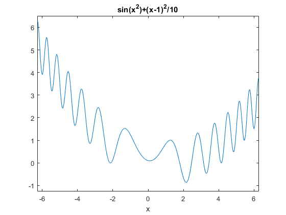
Here the list L of minima consists of one box, and the list Ls of potential minima is empty. Thus the global minimum of f in [-10,10] is enclosed in L with global minimum in mu.

Failure of Matlab for global minimum of univariate function

The Matlab routine fminbnd tries to compute the global minimum of a univariate function, but sometimes fails for simple examples. Consider

f = @(x)cos(x.^2-5)+atan(x)
close
x = linspace(1,4,1e5);
plot(x,f(x),x,0*x)
title('cos(x^2-5)+atan(x)  in  [1,4]')

f =
  function_handle with value:
    @(x)cos(x.^2-5)+atan(x)

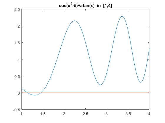
Obviously the global minimum on [1,4] is near x=1.3 as computed by our verification algorithm, however, Matlab's fminbnd fails by picking a local minimum:

[mu,L,Ls] = verifyglobalmin(f,infsup(1,4))
Y = fminbnd(f,1,4)

intval mu = 
  -0.07109205522357
intval L = 
   1.31055395864451
Ls =
     []
Y =
   2.849972728820330

Global minima for multivariate functions

Consider Griewank's function, a famous test function in global optimization

close
f = funvec(@(x)( 1 + sum(x.^2)/4000 - cos(x(1))*cos(x(2)/sqrt(2)) ),zeros(2,1))
[x,y] = meshgrid(-600:10:600,-600:10:600);
surf(x,y,reshape(f([x(:) y(:)]'),size(x)))
view(3)
title('Griewank''s function in [-600,600]^2 on a coarse grid')

f =
  function_handle with value:
    @(x)(1+sum(x.^2)./4000-cos(x(1,:)).*cos(x(2,:)./sqrt(2)))

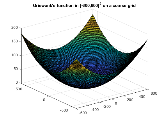
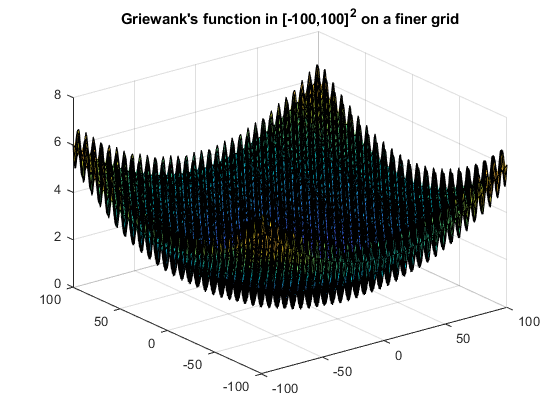
The function on its originally given domain X := [-600,600]^2 looks rather innocent, however a little zooming decovers the nature of the function. Note Griewank's function has more than 200,000 local extrema in X.

close
[x,y] = meshgrid(-100:100,-100:100);
surf(x,y,reshape(f([x(:) y(:)]'),size(x)))
view(3)
title('Griewank''s function in [-100,100]^2 on a finer grid')

The global minimum of Griewank's function is zero with function value zero. It can be verified as follows

format infsup
tic
X = repmat(infsup(-600,600),2,1);
[mu,L,Ls] = verifyglobalmin(@Griewank,X)
toc

intval mu = 
[   0.00000000000000,   0.00000000000000] 
intval L = 
  1.0e-011 *
[  -0.34197302650232,   0.00000000000001] 
[  -0.48338118989294,   0.00000000000001] 
Ls =
     []
Elapsed time is 0.187646 seconds.

Next we display the search boxes of the algorithm.

verifyglobalmin(@Griewank,X,verifyoptimset('Display','~'));
title('Search boxes for the 2-dimensional Griewank function')

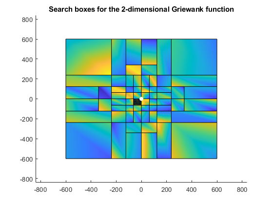
Wide boxes far from the global minimum zero are quickly discarded, whereas more bisections are necessary near the global minimum. Zooming into the plot by a factor 100 shows that granularity of the graph:

zoom(100)
title('Zoom into search boxes for the 2-dimensional Griewank function')

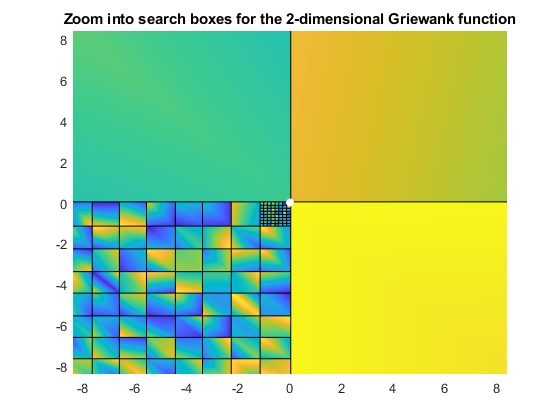
It also becomes clear that we choose a midpoint slightly off the true midpoint. That proves to be efficient because in benchmark examples such as Griewank's function the true global minimum of often on the boundary of bisected intervals. That, however, is unlikely in real-life problems. That lead to the different choice of the midpoint, see

S.M. Rump. Mathematically Rigorous Global Optimization in Floating-Point Arithmetic. to appear in Optimization Methods & Software, 33(4?6):771?798, 2018.

Griewank's n-dimensional test function

Griewank's test function is in fact n-dimensional; it is defined as follows:

n = size(x,1);
y = 1 + sum(x.^2,1)/4000;
p = 1;
for i=1:n
  p = p .* cos(x(i,:)/sqrt(i));
end
y = y - p;

The constraint box is [-600,600]^n, and again the global minimum is the origin. For n=10 the global minimum with a maximum relative tolerance of 1e-5 for the inclusion box is computed as follows:

format infsup long e
tic
X = repmat(infsup(-600,600),10,1);
[mu,L,Ls] = verifyglobalmin(@Griewank,X,verifyoptimset('TolXrel',1e-5))
toc

intval mu = 
[  0.000000000000000e+000,  0.000000000000000e+000] 
intval L = 
[ -9.992007221626428e-036,  9.992007221626428e-036] 
[ -1.332477947954758e-035,  1.654361225119381e-024] 
[ -1.654361225120491e-024,  1.443525429909001e-035] 
[ -8.881784197001268e-036,  8.881784197001268e-036] 
[ -1.110223024625158e-035,  1.110223024625158e-035] 
[ -1.654361225120491e-024,  1.443451961512075e-035] 
[ -1.332459580855527e-035,  1.654361225119381e-024] 
[ -9.992007221626416e-036,  9.992007221626416e-036] 
[ -1.110401351145504e-035,  1.654361225117160e-024] 
[ -1.110223024625157e-035,  1.110223024625157e-035] 
Ls =
     []
Elapsed time is 0.859636 seconds.

Note that the number of local extrema grows exponentially with the dimension. For n=10 there are about 10^29 local extrema in X.

Global minima of a non-smooth function - The Half-Pipe

Consider the half-pipe, a famous test function in non-smooth optimization:

f = @(x) max( x(2,:).^2 - max(x(1,:),0) , 0 )
close
[x,y] = meshgrid(-1:.025:1,-1:.025:1);
surf(x,y,reshape(f([x(:) y(:)]'),size(x)))
view(52,26)
title('The halp-pipe in [-1,1]^2')

f =
  function_handle with value:
    @(x)max(x(2,:).^2-max(x(1,:),0),0)

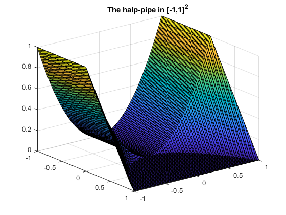
The global minimum of the half-pipe is zero and admitted for all (x,0) with x <= 0 and all (x,y) with 0 <= x <= y^2. Sharp bounds (in fact, the true minimum zero) for the global minimum are computed as well a list of possible minimizers:

[mu,L,Ls,data] = verifyglobalmin(f,infsup(-100,100)*ones(2,1),verifyoptimset('TolXabs',0.5));
mu
infsup(mu)
L
size(Ls)
close
plotintval(Ls)
title('Inclusion of global minima of the half-pipe')

intval mu = 
[  0.000000000000000e+000,  0.000000000000000e+000] 
intval mu = 
[  0.000000000000000e+000,  0.000000000000000e+000] 
L =
     []
ans =
           2       17954

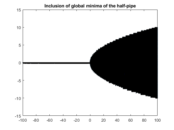
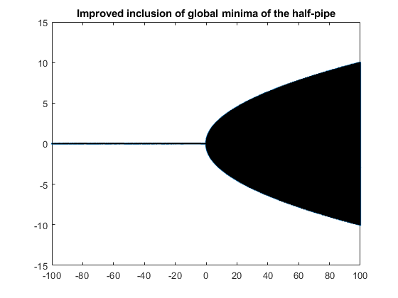
By the principle of verification methods it is not possible to verify a minimizer because that is an ill-posed problem. Therefore, the list L of verified global minima must be empty. The list Ls of potential minimizers can be refined as usual:

[mu,L,Ls,data] = verifyglobalmin(data);
mu
size(Ls)
close
plotintval(Ls)
title('Improved inclusion of global minima of the half-pipe')

intval mu = 
[  0.000000000000000e+000,  0.000000000000000e+000] 
ans =
           2      275813

Infinite boxes

As has been seen in some example above, in principle a box constraint may consist of infinite intervals. However, this is not working in general. Consider

f = @(x)(x^3-x)

f =
  function_handle with value:
    @(x)(x^3-x)

Obviously that function has the three simple roots -1, 0 and 1. Thus one may expect no problems when computing all roots in some box, say [-10,10]:

format long _
X = infsup(-10,10);
[L,Ls] = verifynlssall(f,X)

intval L = 
  -1.00000000000000   0.00000000000000   1.00000000000000
Ls =
     []

Indeed that is an easy task. However, specifying the real axis for X results in

format long e infsup
X = infsup(-inf,inf);
[L,Ls] = verifynlssall(f,X);
L = L'
Ls = Ls'

intval L = 
[ -1.000000000000001e+000, -9.999999999999998e-001] 
[  9.999999999999998e-001,  1.000000000000001e+000] 
[ -2.220446049250314e-036,  2.220446049250314e-036] 
intval Ls = 
[                   - Inf, -8.627484236379337e+155] 
[  8.627484236379337e+155,                     Inf] 

Now inclusions of the roots -1, 0 and 1 are computed as before, however, two infinite boxes covering the negative and positive infinite range remain. The reason is that f(Y)=[-inf,inf] for any real r and Y=[-inf,r] or [r,inf]. Knowing only the function handle of f, there is no better answer.

Roots on the boundary of a box

As a principle of verification methods, roots on the boundary of a constraint box cannot be included. Except special cases, an inclusion of a root is always an interval with nonempty diameter. Thus, it cannot be decided whether the true root is within the box constraint or not. Consider

format long
f = @(x)(x^2 - 4)
[L,Ls] = verifynlssall(f,infsup(-2,2))

f =
  function_handle with value:
    @(x)(x^2-4)
L =
     []
intval Ls = 
[  -2.00000000000000,  -1.99999999928283] [   1.99999999919033,   2.00000000000000] 

The situation changes if the box is widened, for example

X = infsup(-2,succ(2));
[L,Ls] = verifynlssall(f,X)

intval L = 
[   1.99999999999999,   2.00000000000001] 
intval Ls = 
[  -2.00000000000000,  -1.99999999928283] 

The root -2 is still on the boundary, but the root +2 is in the inner of the input box X. Thus an inclusion of +2 is on the new list L, the boundary root -2 still on Ls. With a little more widening of X, the list L contains both -2 and +2, whereas Ls is empty.

Minima on the boundary of a box

Consider minimizing f(x)=(x-1)^2 on X=[-1,1]. We reformulate the function to make sure that rounding error occur, even when evaluating f(1):

f = @(x) sum(x/3.*(3*x-6)+1,1)
X = infsup(-1,1)*ones(2,1)

f =
  function_handle with value:
    @(x)sum(x/3.*(3*x-6)+1,1)
intval X = 
[  -1.00000000000000,   1.00000000000000] 
[  -1.00000000000000,   1.00000000000000] 

Obviously the global minimum is x = [ 1 ; 1 ], which is on the boundary of X. The global minimum is found by

[mu,L,Ls] = verifyglobalmin(f,X)

intval mu = 
  1.0e-007 *
[  -0.64281208578266,   0.00000000222045] 
L =
     []
intval Ls = 
  Columns 1 through 2
[   0.99999999995386,   1.00000000000000] [   0.99999996883388,   0.99999996883389] 
[   0.99999999990483,   1.00000000000000] [   0.99999993571879,   1.00000000000000] 
  Columns 3 through 4
[   0.99999993571879,   1.00000000000000] [   0.99999993571879,   0.99999993571880] 
[   0.99999993571879,   0.99999993571880] [   0.99999993571879,   1.00000000000000] 
  Columns 5 through 6
[   0.99999999267377,   1.00000000000000] [   0.99999998889960,   0.99999998889961] 
[   0.99999998889960,   0.99999998889961] [   0.99999999267377,   1.00000000000000] 
  Columns 7 through 8
[   0.99999999267377,   1.00000000000000] [   0.99999998111523,   0.99999998111524] 
[   0.99999998111523,   0.99999998111524] [   0.99999999267377,   1.00000000000000] 
  Columns 9 through 10
[   0.99999999267377,   1.00000000000000] [   0.99999997710504,   0.99999997710505] 
[   0.99999997710504,   0.99999997710505] [   0.99999999267377,   1.00000000000000] 
  Columns 11 through 12
[   0.99999999644795,   0.99999999644796] [   0.99999999267377,   1.00000000000000] 
[   0.99999999267377,   1.00000000000000] [   0.99999999267377,   0.99999999267378] 
  Columns 13 through 14
[   0.99999999267377,   0.99999999267378] [   0.99999999267377,   1.00000000000000] 
[   0.99999999267377,   1.00000000000000] [   0.99999998488941,   0.99999998488942] 
  Columns 15 through 16
[   0.99999998488941,   0.99999998488942] [   0.99999999916502,   1.00000000000000] 
[   0.99999999267377,   1.00000000000000] [   0.99999999318977,   0.99999999318978] 
  Columns 17 through 18
[   0.99999999916502,   1.00000000000000] [   0.99999999916502,   1.00000000000000] 
[   0.99999999510371,   0.99999999510372] [   0.99999999416103,   0.99999999416104] 
  Columns 19 through 20
[   0.99999999916502,   1.00000000000000] [   0.99999999916502,   1.00000000000000] 
[   0.99999999367540,   0.99999999367541] [   0.99999999693358,   0.99999999693359] 
  Columns 21 through 22
[   0.99999999693358,   0.99999999693359] [   0.99999999916502,   1.00000000000000] 
[   0.99999999916502,   1.00000000000000] [   0.99999999784767,   0.99999999784768] 
  Columns 23 through 24
[   0.99999999784767,   0.99999999784768] [   0.99999999916502,   1.00000000000000] 
[   0.99999999916502,   1.00000000000000] [   0.99999999739062,   0.99999999739064] 
  Columns 25 through 26
[   0.99999999739062,   0.99999999739064] [   0.99999999916502,   1.00000000000000] 
[   0.99999999916502,   1.00000000000000] [   0.99999999556075,   0.99999999556076] 
  Columns 27 through 28
[   0.99999999916502,   1.00000000000000] [   0.99999999916502,   1.00000000000000] 
[   0.99999999461808,   0.99999999461809] [   0.99999999873487,   0.99999999873488] 
  Columns 29 through 30
[   0.99999999873487,   0.99999999873488] [   0.99999999916502,   1.00000000000000] 
[   0.99999999916502,   1.00000000000000] [   0.99999999601780,   0.99999999601781] 
  Columns 31 through 32
[   0.99999999916502,   1.00000000000000] [   0.99999999827782,   0.99999999827783] 
[   0.99999999827782,   0.99999999827783] [   0.99999999916502,   1.00000000000000] 
  Columns 33 through 34
[   0.99999999959516,   0.99999999959517] [   0.99999999916502,   1.00000000000000] 
[   0.99999999916502,   1.00000000000000] [   0.99999999916502,   0.99999999916503] 
  Columns 35 through 36
[   0.99999999916502,   0.99999999916503] [   0.99999999916502,   1.00000000000000] 
[   0.99999999916502,   1.00000000000000] [   0.99999999644795,   0.99999999644796] 
  Columns 37 through 38
[   0.99999999990483,   1.00000000000000] [   0.99999999990483,   1.00000000000000] 
[   0.99999999922382,   0.99999999922383] [   0.99999999944196,   0.99999999944197] 
  Columns 39 through 40
[   0.99999999990483,   1.00000000000000] [   0.99999999965051,   0.99999999965052] 
[   0.99999999965051,   0.99999999965052] [   0.99999999990483,   1.00000000000000] 
  Columns 41 through 42
[   0.99999999990483,   1.00000000000000] [   0.99999999990483,   1.00000000000000] 
[   0.99999999933452,   0.99999999933453] [   0.99999999927917,   0.99999999927918] 
  Columns 43 through 44
[   0.99999999990483,   1.00000000000000] [   0.99999999985581,   0.99999999985582] 
[   0.99999999985581,   0.99999999985582] [   0.99999999990483,   1.00000000000000] 
  Columns 45 through 46
[   0.99999999990483,   1.00000000000000] [   0.99999999975469,   0.99999999975470] 
[   0.99999999975469,   0.99999999975470] [   0.99999999990483,   1.00000000000000] 
  Columns 47 through 48
[   0.99999999990483,   1.00000000000000] [   0.99999999990483,   1.00000000000000] 
[   0.99999999954614,   0.99999999954615] [   0.99999999970260,   0.99999999970261] 
  Columns 49 through 50
[   0.99999999970260,   0.99999999970261] [   0.99999999990483,   1.00000000000000] 
[   0.99999999990483,   1.00000000000000] [   0.99999999949405,   0.99999999949406] 
  Columns 51 through 52
[   0.99999999990483,   1.00000000000000] [   0.99999999990483,   1.00000000000000] 
[   0.99999999938661,   0.99999999938662] [   0.99999999990483,   0.99999999990484] 
  Columns 53 through 54
[   0.99999999990483,   0.99999999990484] [   0.99999999990483,   1.00000000000000] 
[   0.99999999990483,   1.00000000000000] [   0.99999999980372,   0.99999999980373] 
  Columns 55 through 56
[   0.99999999980372,   0.99999999980373] [   0.99999999990483,   1.00000000000000] 
[   0.99999999990483,   1.00000000000000] [   0.99999999959516,   0.99999999959517] 
  Column 57
[   0.99999999995386,   0.99999999995387] 
[   0.99999999990483,   1.00000000000000] 

The list L is empty because the minimum x=1 is on the boundary of X and, by principle of verification methods, it cannot be verified that f'(x) has a root in X. The inclusion mu of the minimum is narrow.

Minima on the boundary of a box for constraint minimization

Consider minimizing f(x) for g(x)=0 on X for

f = @(x)(x)
g = @(x)(cos(2*atan(x)))
X = infsup(-1,1)

f =
  function_handle with value:
    @(x)(x)
g =
  function_handle with value:
    @(x)(cos(2*atan(x)))
intval X = 
[  -1.00000000000000,   1.00000000000000] 

Since 4*atan(1)=pi, there are exactly two feasible points -1 and 1, both on the boundary of X. Thus, the minimum value of the trivial function f is -1. However,

[mu,L,Ls] = verifyconstraintglobalmin(f,g,X)

intval mu = 
[  -1.00000000000000,                Inf] 
L =
     []
intval Ls = 
[  -1.00000000000000,  -0.99930399065472] [   0.99921421872424,   1.00000000000000] 

According to the specification of verifyconstraintglobalmin, each box in the list L consists of a local minimum of f, on Ls are possible inclusions. Thus the wide inclusion mu of the minimum value is true, but with the upper bound inf it seems very week.

However, given the information at hand, that is the best possible information we can obtain. Since -1 and 1 are on the boundary of X, it can not be verified whether the feasible region is empty of not. Thus the minimum of f(X), without constraint, is the best information about the minimum of f s.t. g(x)=0.

However, no better upper bound than +inf for the minimum is possible. That is because if the feasible region were empty, convention says that the minimum is +inf, and that is the upper bound of mu.

Widening the box on the right allows at least to verify existence of a feasible point

format infsup
X = infsup(-1,succ(1,2));
[mu1,L1,Ls1] = verifyconstraintglobalmin(f,g,X)

intval mu1 = 
[  -1.00000000000000,   1.00000000000001] 
intval L1 = 
[   0.99999999999999,   1.00000000000001] 
intval Ls1 = 
[  -1.00000000000000,  -0.99999999998018] 

This reduces mu to about [-1,1]. Since -1 is still on the boundary, it cannot be verified to be feasible. Finally, widening the box X on both sides moves both feasible points to the interior and the result is as anticipated.

e = 1e-14;
X = infsup(-1-e,1+e);
[mu2,L2,Ls2] = verifyconstraintglobalmin(f,g,X)

intval mu2 = 
[  -1.00000000000002,  -0.99999999999999] 
intval L2 = 
[  -1.00000000000001,  -0.99999999999999] 
Ls2 =
     []

Finding all roots of the gradient

For a given function f:R^n->R all roots of the gradient within a box X can be computed, i.e., all stationary points. Consider

format short
n = 3;
X = infsup(-10,10)*ones(n,1);
tic
[L,Ls] = verifynlssderivall(@Griewank,X,verifynlssallset('iFunMax',1e6));
tDerivall = toc
size(L)
size(Ls)

tDerivall =
    1.9131
ans =
     3   265
ans =
     0     0

That means there are 265 stationary points of the Griewank function within the box [-10,10]^3. Another way to produce that result is to compute explicitly given gradient of the Griewank function in some function Griewanks:

tic
[L1,Ls1] = verifynlssall(@Griewanks,X,verifynlssallset('iFunMax',1e6));
tnlssall = toc
size(L1)
size(Ls1)

tnlssall =
    2.0057
ans =
     3   265
ans =
     0     0

Rigorous range estimation

Given a function f:R^n->R^m and some box X in IR^n, f(X) computes an inclusion of the range of f over X. For example,

format short
f = @(x) sin(2*x.^2./sqrt(cosh(x))-x) - atan(4*x+1) + 1
X = infsup(0,4)
Y = f(X)

f =
  function_handle with value:
    @(x)sin(2*x.^2./sqrt(cosh(x))-x)-atan(4*x+1)+1
intval X = 
[    0.0000,    4.0000] 
intval Y = 
[   -1.5121,    1.2147] 

By definition, Y is an outer inclusion of the range of f over X. A more refined range estimation is calculated by verifyrange:

[ Yout , Yin ] = verifyrange(f,X)

intval Yout = 
[   -0.2967,    0.5657] 
intval Yin = 
[   -0.2959,    0.5656] 

Here Yout is an outer inclusion of f over X, Yin an inner inclusion. For that example, Yout and Y are not too far apart. However, only from Y we cannot deduce whether f has a root in X or not, but the inner inclusion Yin proves that f has indeed a root in X.

The example is taken from my Acta Numerica article to demonstrate drastic overestimation. In fact, change the sin into sinh over the same box X:

f2 = @(x) sinh(2*x.^2./sqrt(cosh(x))-x) - atan(4*x+1) + 1
Y2 = f2(X)

f2 =
  function_handle with value:
    @(x)sinh(2*x.^2./sqrt(cosh(x))-x)-atan(4*x+1)+1
intval Y2 = 
  1.0e+013 *
[   -0.0001,    3.9482] 

The computed interval Y2 is an inclusion of the range of f2, however, it is not clear how much overestimation took place. That can be checked with verifyrange:

[ Yout2 , Yin2 ] = verifyrange(f2,X)

intval Yout2 = 
[   -0.2966,    6.7265] 
intval Yin2 = 
[   -0.2962,    6.7189] 

The problem is that the argument 2*x.^2./sqrt(cosh(x))-x of the sinh causes much dependencies for x=infsup(0,4):

2*X.^2./sqrt(cosh(X)) - X

intval ans = 
[   -4.0000,   32.0000] 

The true range of the function can also be seen from the graph:

x = linspace(0,4,1000);
close
plot(x,f2(x),x,0*x)
title('sinh(2x^2/sqrt(cosh(x))-x) - atan(4x+1) + 1  in  [0,4]')

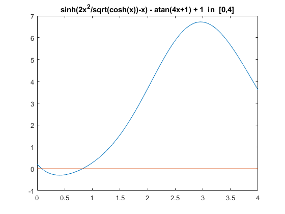
The graph shows how drastic the overestimation by standard interval arithmetic is in that constructed example. From the graph there is also numerical evidence that the inclusion Yout2 is almost sharp.

If the accuracy is not sufficient, it can be improved using another method, for example global optimization:

[ Yout3 , Yin3 ] = verifyrange(f2,X,verifyrangeset('Method','globopt'))
format long
Yout3
Yin3

intval Yout3 = 
[   -0.2962,    6.7189] 
intval Yin3 = 
[   -0.2962,    6.7189] 
intval Yout3 = 
[  -0.29610750359467,   6.71886053894845] 
intval Yin3 = 
[  -0.29610750359465,   6.71886053894677] 

The inner inclusion hardly changed, but the outer became much narrower, almost equal to the inner inclusion. That identifies the range very precisely.

Parameter identification

Let a function f and a box X be given. Parameter identification means to find for a given interval P all x in X with the property that f(x) is in P. The interval P may be a point.

As an example, consider to find the zero set of

f = -(5*y - 20*y^3 + 16*y^5)^6 + (-(5*x - 20*x^3 + 16*x^5)^3 + 5*y - 20*y^3 + 16*y^5)^2

on the box X = infsup(-1,1)^2:

f = @(x) -(5*x(2) - 20*x(2)^3 + 16*x(2)^5)^6 + (-(5*x(1) - 20*x(1)^3 + 16*x(1)^5)^3 + 5*x(2) - 20*x(2)^3 + 16*x(2)^5)^2;
X = infsup(-1,1)*ones(2,1);
format short
tic
verifynlssparam(f,0,X,verifynlssparamset('Display','~'));
tIntval = toc
title('Parameter identification - default setting')

tIntval =
    0.3261

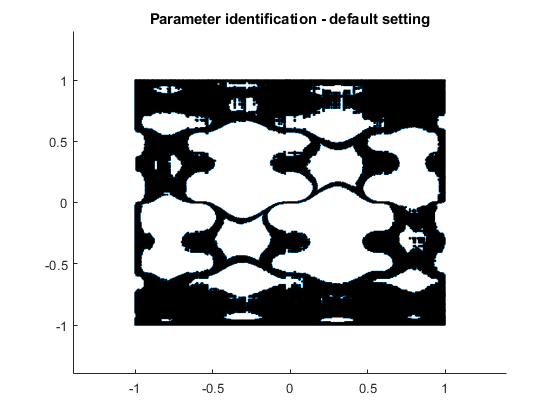
As a principal limit, it cannot be verified that the value of a function is truly zero. However, certain areas can be excluded, and in the graph these are the white areas. The black area are potential members of the zero set.

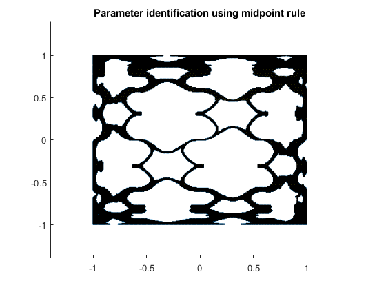
Parameter identification using the midpoint rule

Due to overestimation by interval arithmetic, the black area is quite big. That can be improved by using the midpoint rule with moderately increasing computing time.

tic
verifynlssparam(f,0,X,verifynlssparamset('Display','~','Method','midrule'));
tMidrule = toc
title('Parameter identification using midpoint rule')

tMidrule =
    0.7192

Parameter identification using affine arithmetic

The picture will be further improved by using affine arithmetic.

tic
verifynlssparam(f,0,X,verifynlssparamset('Display','~','Method','affari'));
tAffari = toc
title('Parameter identification using affine arithmetic')

tAffari =
    6.0285

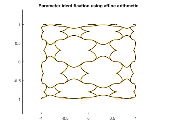
However, the improvement comes with significantly increased computing time.

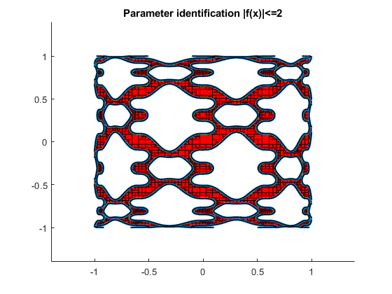
When widening P, for example displaying all x in X such that abs(f(x))<=0.2, also red areas appear. That covers points definitely satisfying the desired property.

verifynlssparam(f,infsup(-0.2,0.2),X,verifynlssparamset('Display','~','Method','affari'));
title('Parameter identification |f(x)|<=2')

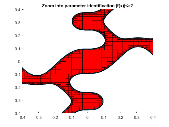
A typical cut section looks as follows, where only the yellow areas are undecided.

axis([-0.4 0.4 -0.4 0.4])
title('Zoom into parameter identification |f(x)|<=2')

Zero areas of non-smooth functions

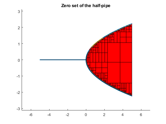
Consider again the half-pipe, a famous test function in non-smooth optimization. As has been mentioned, the half-pipe is entirely zero for all (x,0) with x <= 0 and all (x,y) with 0 <= x <= y^2. Now the zero regions are not only one-dimensional, so that red areas appear although testing for f(x)=0:

f = @(x) max( x(2,:).^2 - max(x(1,:),0) , 0 )
X = infsup(-5,5)*ones(2,1)
verifynlssparam(f,0,X,verifynlssparamset('Display','~'));
title('Zero set of the half-pipe')

f =
  function_handle with value:
    @(x)max(x(2,:).^2-max(x(1,:),0),0)
intval X = 
[   -5.0000,    5.0000] 
[   -5.0000,    5.0000] 

A 4-dimensional parameter identification problem with 2 parameters

Finally we show a parameter identification we found in the literature:

f = @(p) [ p(1,:).*exp(0.2*p(2,:)) ;
           p(1,:).*exp(p(2,:)) ;
           p(1,:).*exp(2*p(2,:)) ;
           p(1,:).*exp(4*p(2,:)) ]
X = infsup(-3,3)*ones(2,1);
P = infsup([1.5 .7 .1 -.1]',[2 .8 .3 .03]')
tic
verifynlssparam(f,P,X,verifynlssparamset('Display','~'));
toc

f =
  function_handle with value:
    @(p)[p(1,:).*exp(0.2*p(2,:));p(1,:).*exp(p(2,:));p(1,:).*exp(2*p(2,:));p(1,:).*exp(4*p(2,:))]
intval P = 
[    1.5000,    2.0000] 
[    0.6999,    0.8001] 
[    0.1000,    0.3000] 
[   -0.1001,    0.0300] 
Elapsed time is 0.563622 seconds.

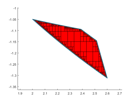
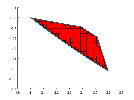
A zoom into the feasible parameter set is as follows:

axis([1.9 2.7 -1.4 -1])

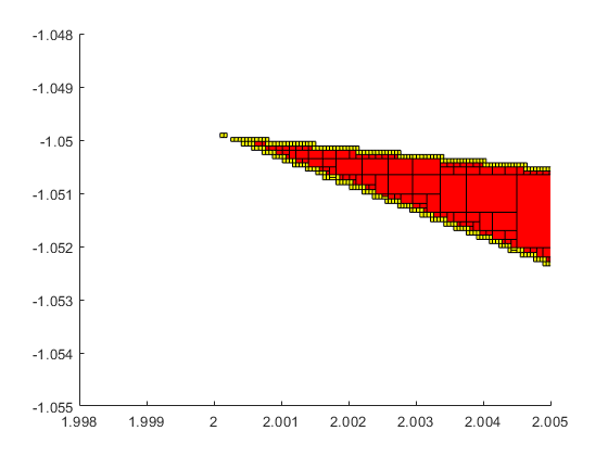
and a further zoom into the upper left corner is as follows:

axis([1.998 2.005 -1.055 -1.048])

In this case the picture does not change much when using the midrule or affine arithmetic.

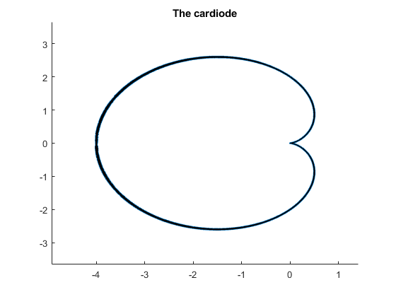
Display of a cardiode

To display a cardiode we use the definition

c = @(x) sqr(sum(sqr(x),1))+4*x(1,:).*sum(sqr(x),1)-4*sqr(x(2,:))

c =
  function_handle with value:
    @(x)sqr(sum(sqr(x),1))+4*x(1,:).*sum(sqr(x),1)-4*sqr(x(2,:))

Then it is straightforward to display the graph, that is the zero set of c(x).

verifynlssparam(c,0,[infsup(-5,1);infsup(-3,3)],verifynlssparamset('display','~'));
title('The cardiode')

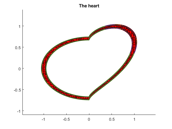
For a nicer heart curve, consider

f = @(x)sqr(x(1,:))+2*sqr(0.6*x(1,:).^(2/3)-x(2,:))-1

f =
  function_handle with value:
    @(x)sqr(x(1,:))+2*sqr(0.6*x(1,:).^(2/3)-x(2,:))-1

Then the set of values with absolute value less than or equal to 0.1 looks as follows.

verifynlssparam(f,midrad(0,.1),midrad(0,1.2)*ones(2,1),verifynlssparamset('display','~'));
title('The heart')

Enjoy INTLAB

INTLAB was designed and written by S.M. Rump, head of the Institute for Reliable Computing, Hamburg University of Technology. Suggestions are always welcome to rump (at) tuhh.de

Published with MATLAB® R2020a