DEMOGFP A short demonstration of gfp-numbers, elements of GF[p]
Contents
Initialization
This toolbox implements arithmetical and other operation in GF[p], not GF[p^n], i.e. it is basically a modulo p arithmetic. To initialize the prime number p, use
p = 7;
gfpinit(p)
Galois field prime set to 7
ans =
     7
The prime number p is limited by 2*p^2<=2^53, i.e. p <= 2^26 = 67,108,864. To retrieve the current prime, use
current_prime = gfpinit
Galois field prime set to 7
current_prime =
     7
Basic operations
The four basic operations are executed as usual, for example, an addition table is as follows:
v = gfp(0:p-1);
add_table = v'+v
gfp add_table =
     0     1     2     3     4     5     6
     1     2     3     4     5     6     0
     2     3     4     5     6     0     1
     3     4     5     6     0     1     2
     4     5     6     0     1     2     3
     5     6     0     1     2     3     4
     6     0     1     2     3     4     5
Similarly, a multiplication table is obtained by
mul_table = v'*v
gfp mul_table =
     0     0     0     0     0     0     0
     0     1     2     3     4     5     6
     0     2     4     6     1     3     5
     0     3     6     2     5     1     4
     0     4     1     5     2     6     3
     0     5     3     1     6     4     2
     0     6     5     4     3     2     1
The reciprocal
As GF[p] being a field, every nonzero number has a unique reciprocal. One way to obtain the reciprocal is the first row of the division table:
v = gfp(1:p-1);
div_table = v'*(1./v)
gfp div_table =
     1     4     5     2     3     6
     2     1     3     4     6     5
     3     5     1     6     2     4
     4     2     6     1     5     3
     5     6     4     3     1     2
     6     3     2     5     4     1
or directly by
reciprocal = 1./v
gfp reciprocal =
     1     4     5     2     3     6
The reciprocal can also be obtained by Fermat's small theorem x^(p-1) = 1, so that x^(p-2) must be the reciprocal of x:
v^(p-2)
gfp ans =
     1     4     5     2     3     6
Conversion of floating-point numbers
Every floating-point number is of the form m*2^e for integers m and e. Thus, they can be mapped into GF[p] by (m mod p) * 2^(e mod p):
gfp_pi = gfp(pi)
gfp_e = gfp(exp(1))
gfp gfp_pi =
     0
gfp gfp_e =
     4
The latter formula can be used for any odd prime; for p=2 and m=m'*2^f we use (m' mod p) * 2^(e+f). Obviously the result is zero except for odd integers.
primitive element
Every field has at least one primitive element, i.e. a generator of the multiplicative group. Using
powers = repmat(gfp(2:p-1)',1,p-2).^repmat(1:p-2,p-2,1)
gfp powers =
     2     4     1     2     4
     3     2     6     4     5
     4     2     1     4     2
     5     4     6     2     3
     6     1     6     1     6
generates all powers of 1..p-1 in the columns of powers. Each row not containing a 1 is a primitive element:
prim_elem = find(all(powers~=1,2))+1
prim_elem =
     3
     5
Indeed the powers are all elements 1..p-1:
gfp(prim_elem(1)) ^ (1:p-1)
gfp(prim_elem(2)) ^ (1:p-1)
gfp ans =
     3     2     6     4     5     1
gfp ans =
     5     4     6     2     3     1
Matrix routines
Operations in GF[p] are always exact, neither rounding errors nor overflow or underflow may occur. Thus the term "ill-conditioned" does not apply. For arbitrarily ill-conditioned matrices it can be proved that they are regular if the determinant mod p is nonzero. Consider
gfpinit(11)
n = 5;
A = invhilb(n)
[L,U,perm] = luwpp(gfp(A));
residual = L*U - A(perm,:)
det_ = prod(diag(U))
Galois field prime set to 11
ans =
    11
A =
          25        -300        1050       -1400         630
        -300        4800      -18900       26880      -12600
        1050      -18900       79380     -117600       56700
       -1400       26880     -117600      179200      -88200
         630      -12600       56700      -88200       44100
gfp residual =
     0     0     0     0     0
     0     0     0     0     0
     0     0     0     0     0
     0     0     0     0     0
     0     0     0     0     0
gfp det_ =
     2
The routine luwpp performs an LU-decomposition of A with partial pivoting. Thus, if det_ is nonzero, the matrix is A is regular. With the small prime p=11 that approach does not work for the inverse Hilbert matrix of dimension 6 because it contains a zero row and column:
A6 = gfp(invhilb(6))
gfp A6 =
     3     8     5     8     3     0
     8     4     9     7     6     0
     5     9     4     1     6     0
     8     7     1    10     9     0
     3     6     6     9     1     0
     0     0     0     0     0     0
The true Hilbert matrix in GF[p]
Alternatively one may define H to be the true Hilbert matrix in GF[p]. Consider H_5 in GF[11]:
n = 5;
gfpinit(11);
H = ( 1:n )' + ( 1:n) - 1
H = 1 ./ gfp(H)
Galois field prime set to 11
H =
     1     2     3     4     5
     2     3     4     5     6
     3     4     5     6     7
     4     5     6     7     8
     5     6     7     8     9
gfp H =
     1     6     4     3     9
     6     4     3     9     2
     4     3     9     2     8
     3     9     2     8     7
     9     2     8     7     5
That matrix is regular in GF[11]:
d = det(H)
gfp d =
     6
Hence there is a unique inverse:
R = inv(H)
R*H
gfp R =
     3     8     5     8     3
     8     4     9     7     6
     5     9     4     1     6
     8     7     1    10     9
     3     6     6     9     1
gfp ans =
     1     0     0     0     0
     0     1     0     0     0
     0     0     1     0     0
     0     0     0     1     0
     0     0     0     0     1
The pseudoinverse
While a matrix being regular in GF[p] has a unique inverse in GF[p], the corresponding theorem is not true for the pseudoinverse. It is not difficult to see that A=[1 3] has no pseudoinverse in GF[5]. While 0.1*[1;3] is the pseudoinverse over R, also a brute-force test demonstrates that there is no pseudoinverse in GF[5]:
gfpinit(5);
A = [1 3];
for i=0:4
  for j=0:4
    P = gfp([i;j]);
    if A * P == 1
      P
      PA = P*A
      disp(' ')
    end
  end
end
Galois field prime set to 5
gfp P =
     0
     2
gfp PA =
     0     0
     2     1

gfp P =
     1
     0
gfp PA =
     1     3
     0     0

gfp P =
     2
     3
gfp PA =
     2     1
     3     4

gfp P =
     3
     1
gfp PA =
     3     4
     1     3

gfp P =
     4
     4
gfp PA =
     4     2
     4     2
The code shows that for all matrices P with A*P=1 implies that P*A is not symmetric. The reason that no pseudoinverse exists, although A has full rank, is that A*A' is not regular:
AAt = gfp(A)*A'
gfp AAt =
     0
Regularity of extremely ill-conditioned matrices
The INTLAB routine "isregular" checks regularity on that basis for extremely ill-conditioned matrices.
Indeed, using a larger prime, very ill-conditioned matrices can be proved to be regular:
gfpinit(67108859)
n = 50;
A = randmat(n,1e200);
C = double( norm(A,inf) * norm(inv(sym(A)),inf) )
[L,U,perm] = luwpp(gfp(A));
det_ = prod(diag(U))
Galois field prime set to 67108859
ans =
    67108859
C =
  2.0541e+223
gfp det_ =
    67108858
In that case we used the largest admissable prime for the gfp-toolbox, so that it is unlikely that the test fails by accident.
Note that the condition number C of the matrix A is computed using the symbolic toolbox of Matlab. That takes some time, but it is reliable.
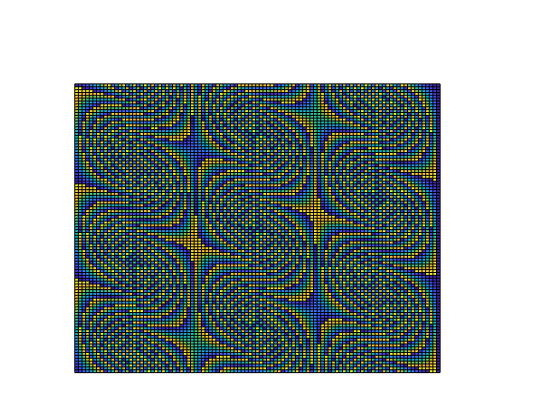
Pictures in GF[p]
For the friends of nice pictures consider
p = 101;
gfpinit(p);
ex = .5*[-1 1 1 -1];
ey = .5*[-1 -1 1 1];
close, hold on
for i=1:p
  for j=1:p
    patch( i+ex , j+ey , double( mod( i^2 + 3*i*j ,p))/p );
  end
end
axis off
hold off
Galois field prime set to 101
Enjoy INTLAB
INTLAB was designed and written by S.M. Rump, head of the Institute for Reliable Computing, Hamburg University of Technology. Suggestions are always welcome to rump (at) tuhh.de