DEMOACCSUMDOT Accurate summation and dot products
The following accurate summation and dot product routines were included in earlier versions of INTLAB. I leave them in INTLAB for upward compatibility. I strongly recommend to use the new functions prodK and spProdK for full and sparse input, included in INTLAB from Version 14, see the demos dprodKand daccmatprod.
Contents
Accurate summation
Some time ago I published various algorithms for the accurate computation of sums and dot products. A typical application is the accurate computation of a residual.
First, define an ill-conditioned matrix, the inverse Hilbert matrix as provided by Matlab (we display only the upper left corner of A):
setround(0)                 % set rounding to nearest
format short

n = 10;
A = invhilb(n);
v = 1:4;
A(v,v)
cond(A)
ans =
   1.0e+09 *
    0.0000   -0.0000    0.0001   -0.0006
   -0.0000    0.0003   -0.0059    0.0476
    0.0001   -0.0059    0.1129   -0.9514
   -0.0006    0.0476   -0.9514    8.2450
ans =
   1.6032e+13
We calculate a right hand side such that the solution is the vector of 1's. Since the matrix entries are not too large integers, the true solution is indeed the vector of 1's.
The approximate solution by the built-in Matlab routine is moderately accurate, as expected by the condition number of the matrix.
format long
b = A*ones(n,1);
xs = A\b
xs =
   1.000000019226368
   1.000000013110664
   1.000000009874403
   1.000000007927763
   1.000000006628883
   1.000000005699745
   1.000000005001583
   1.000000004457446
   1.000000004021206
   1.000000003663520
Residual iteration
If one residual iteration is performed in working precision, Skeel proved that the result becomes backward stable; however, the forward error does not improve. We display the result after five iterations.
for i=1:5
  xs = xs - A\(A*xs-b);
end
xs
xs =
   1.000032535546598
   1.000030117994271
   1.000027868465711
   1.000025853088451
   1.000024068329745
   1.000022490697542
   1.000021093081011
   1.000019850103757
   1.000018739617530
   1.000017742823954
Accurate residual iteration
This changes when calculating the residual in double the working precision. After four iterations the approximation is fully accurate.
for i=1:4
  xs = xs - A\Dot_(A,xs,-1,b);
end
xs
xs =
     1
     1
     1
     1
     1
     1
     1
     1
     1
     1
Note that the residual is calculated "as if" in double the working precision, but the result of the dot product is stored in working precision.
Verified inclusion
The same principle is used in the verification routine verifylss.
X = verifylss(A,b)
rel = relerr(X);
medianmaxrel = [median(rel) max(rel)]
intval X =
   1.00000000000000
   1.00000000000000
   1.00000000000000
   1.00000000000000
   1.00000000000000
   1.00000000000000
   1.00000000000000
   1.00000000000000
   1.00000000000000
   1.00000000000000
medianmaxrel =
     0     0
The inclusion X is a point interval, i.e., all left and bounds coincide:
maxdiamX = max(diam(X))
maxdiamX =
     0
This is an exceptional case due to fact that all entries of A and b are integers.
Very ill-conditioned matrices
Next we use an extremely ill-conditioned matrix proposed by Boothroyd (we show some entries of the upper left corner). As before the right hand side is computed such that the exact solution is the vector of 1's.
n = 15;
[A,Ainv] = boothroyd(n);
A(v,v)
b = A*ones(n,1);
ans =
          15         105         455        1365
         120        1120        5460       17472
         680        7140       37128      123760
        3060       34272      185640      636480
Since the inverse is the original matrix with a checkerboard sign distribution and thus explicitly known, the condition number is just the norm of A squared.
format short
cnd = norm(A)*norm(Ainv)
cnd =
   1.5132e+23
As expected, the Matlab approximation has no correct digit, even the sign is not correct.
xs = A\b
xs =
   1.0e+03 *
    0.0010
    0.0010
    0.0010
    0.0009
    0.0015
   -0.0004
    0.0046
   -0.0066
    0.0145
   -0.0168
    0.0083
    0.0566
   -0.2600
    0.8067
   -2.0890
Using accurate dot products based on error-free transformations, an inclusion of the solution can be calculated:
format long _
X = verifylss(A,b,'illco')
intval X =
   1.00000000000000
   1.00000000000000
   1.00000000000000
   1.0000000000000_
   1.000000000000__
   1.000000000000__
   1.00000000000___
   1.00000000000___
   1.0000000000____
   1.0000000000____
   1.0000000000____
   1.000000000_____
   1.000000000_____
   1.000000000_____
   1.00000000______
Extremely ill-conditioned sums and dot products
There are routines to generate extremely ill-conditioned sums and dot products. Consider
n = 50;
cnd = 1e25;
[x,y,c] = GenDot(n,cnd);
Here x,y are vectors such that the dot product x'*y is extremely ill-conditioned (condition number ~1e25). Hence the accurate computation of x'*y is outside the scope of double precision (binary64) floating-point arithmetic. The outoput parameter c is the exact value of x'*y.
Computation "as if" in K-fold precision
It can be expected that a floating-point approximation has no correct digit, in fact true result and approximation have opposite sign and differ significantly in magnitude:
c
x'*y
c =
   1.262911246333432
ans =
   251527168
The computation of x'*y in double the working precision gives a more accurate approximation:
c
Dot_(x',y)
c =
   1.262911246333432
ans =
   1.262911260128021
A result "as if" computed in triple the working precision and rounded into working precision is accurate to the last bit:
c
Dot_(x',y,3)
c =
   1.262911246333432
ans =
   1.262911246333432
Accurate approximation
An alternative is to use error-free transformations to compute faithfully rounded results, independent of the condition number. For an extremely ill-conditioned dot product with condition number 1e100 the result is still accurate to the last bit.
n = 50;
cnd = 1e100;
[x,y,c] = GenDot(n,cnd);
c
AccDot(x',y)
c =
   0.415696163779104
ans =
   0.415696163779104
An inclusion of the result can be computed as well:
c
infsup(AccDot(x',y,[]))
c =
   0.415696163779104
intval  =
[   0.41569616377910,   0.41569616377911]
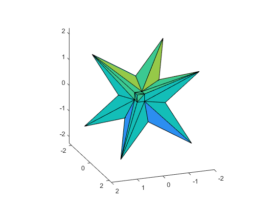
Hidden line
There is quite some effort in computer geometry to design properly working hidden line algorithms. The decision whether a point is visible or not is decided by the sign of some dot product. It seems hard to believe, but evaluating dot products in double precision is sometimes not enough to make the correct decision and pictures are blurred. In that case an accurate dot product may help.
The following graph shows the solution set of an interval linear system as on the cover of Arnold's book. When executing this in Matlab and rotating the graph, sometimes the display is not correct.
format short
A = ones(3)*infsup(0,2); A(1:4:end) = 3.5
b = ones(3,1)*infsup(-1,1)
plotlinsol(A,b)
view(-200,20)
intval A =
[    3.5000,    3.5000] [    0.0000,    2.0000] [    0.0000,    2.0000]
[    0.0000,    2.0000] [    3.5000,    3.5000] [    0.0000,    2.0000]
[    0.0000,    2.0000] [    0.0000,    2.0000] [    3.5000,    3.5000]
intval b =
[   -1.0000,    1.0000]
[   -1.0000,    1.0000]
[   -1.0000,    1.0000]
intval ans =
[   -1.7648,    1.7648]
[   -1.7648,    1.7648]
[   -1.7648,    1.7648]
Enjoy INTLAB
INTLAB was designed and written by S.M. Rump, head of the Institute for Reliable Computing, Hamburg University of Technology. Suggestions are always welcome to rump (at) tuhh.de